Independent Samples Comparing Proportions Lecture 37 Section 11

Independent Samples: Comparing Proportions Lecture 37 Section 11. 5 Tue, Nov 6, 2007

Comparing Proportions We wish to compare proportions between two populations. n We should compare proportions for the same attribute in order for it to make sense. n ¨ For example, we could measure the proportion of NC residents living below the poverty level and the proportion of VA residents living below the poverty level.

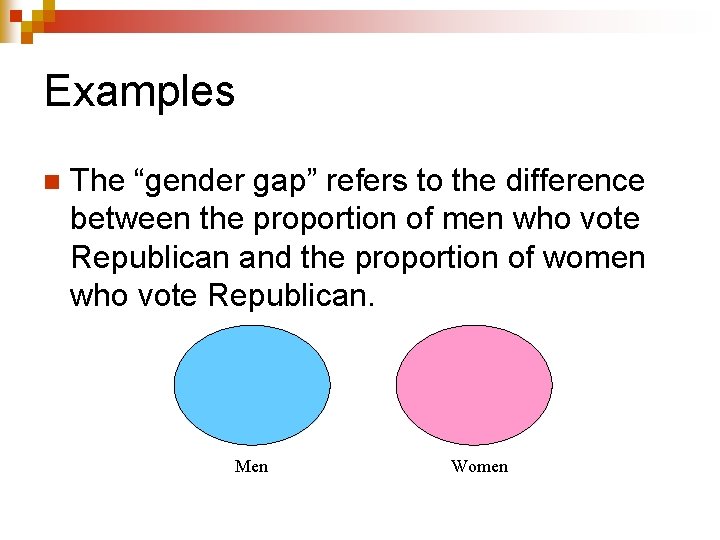
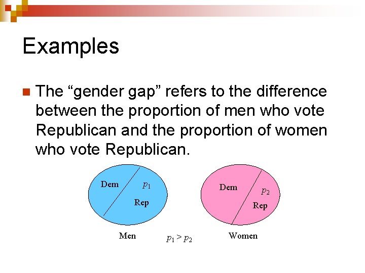
Examples n The “gender gap” refers to the difference between the proportion of men who vote Republican and the proportion of women who vote Republican. Men Women

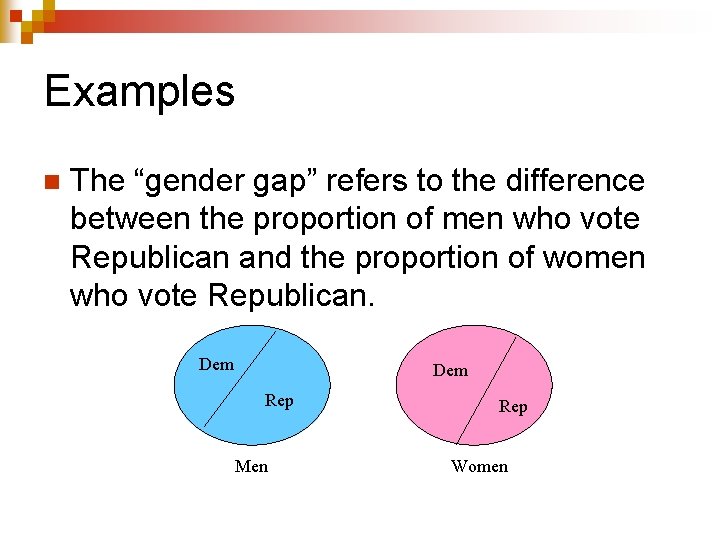
Examples n The “gender gap” refers to the difference between the proportion of men who vote Republican and the proportion of women who vote Republican. Dem Rep Men Rep Women

Examples n The “gender gap” refers to the difference between the proportion of men who vote Republican and the proportion of women who vote Republican. p 1 Dem Rep Men p 2 Rep p 1 > p 2 Women

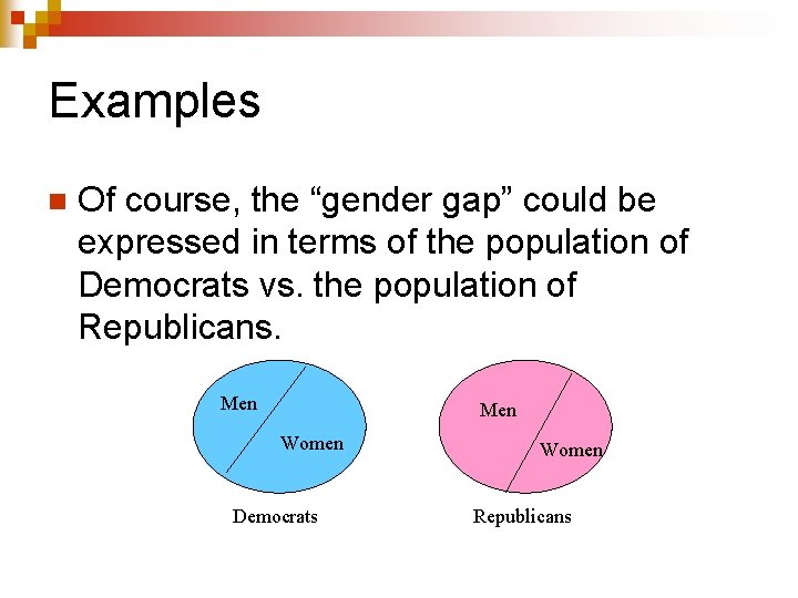
Examples n Of course, the “gender gap” could be expressed in terms of the population of Democrats vs. the population of Republicans. Men Women Democrats Women Republicans

Examples n The proportion of patients who recovered, given treatment A vs. the proportion of patients who recovered, given treatment B. ¨ p 1 = recovery rate under treatment A. ¨ p 2 = recovery rate under treatment B.

Comparing proportions To estimate the difference between population proportions p 1 and p 2, we need the sample proportions p 1^ and p 2^. n The sample difference p 1^ – p 2^ is an estimator of the true difference p 1 – p 2. n

Case Study 13 City Hall turmoil: Richmond Times. Dispatch poll. n Test the hypothesis that a higher proportion of men than women believe that Mayor Wilder is doing a good or excellent job as mayor of Richmond. n

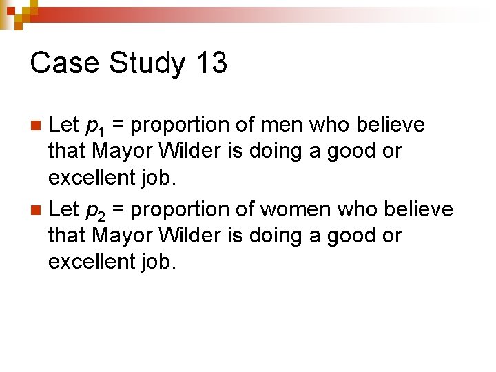
Case Study 13 Let p 1 = proportion of men who believe that Mayor Wilder is doing a good or excellent job. n Let p 2 = proportion of women who believe that Mayor Wilder is doing a good or excellent job. n

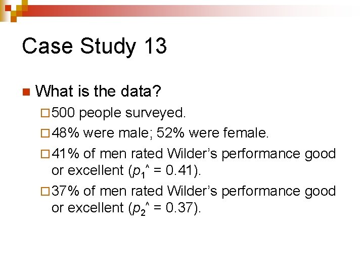
Case Study 13 n What is the data? ¨ 500 people surveyed. ¨ 48% were male; 52% were female. ¨ 41% of men rated Wilder’s performance good or excellent (p 1^ = 0. 41). ¨ 37% of men rated Wilder’s performance good or excellent (p 2^ = 0. 37).

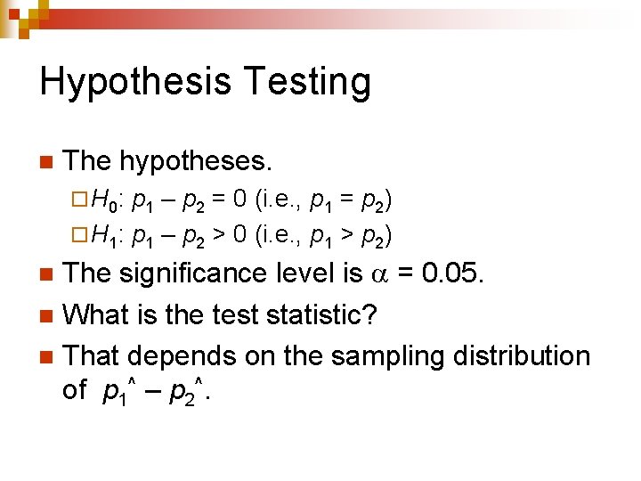
Hypothesis Testing n The hypotheses. ¨ H 0: p 1 – p 2 = 0 (i. e. , p 1 = p 2) ¨ H 1: p 1 – p 2 > 0 (i. e. , p 1 > p 2) The significance level is = 0. 05. n What is the test statistic? n That depends on the sampling distribution of p 1^ – p 2^. n

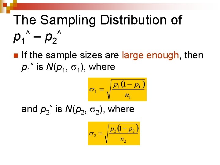
The Sampling Distribution of ^ ^ p 1 – p 2 n If the sample sizes are large enough, then p 1^ is N(p 1, 1), where and p 2^ is N(p 2, 2), where

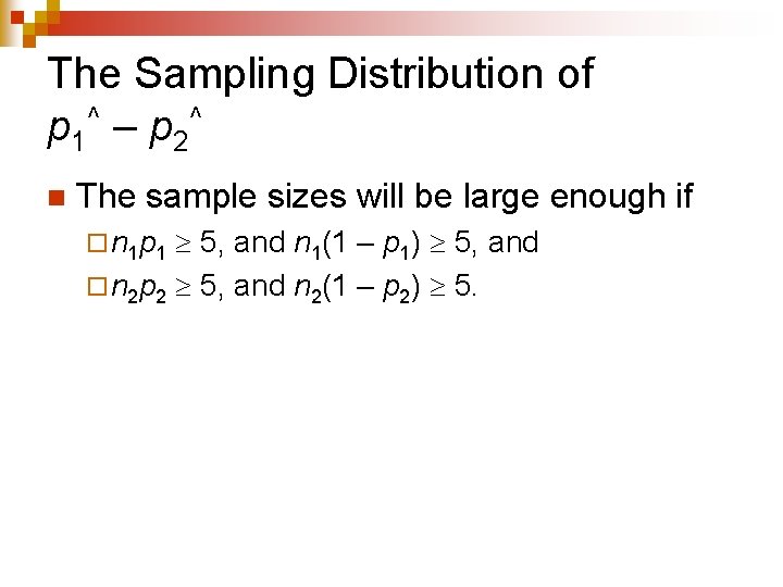
The Sampling Distribution of p 1^ – p 2^ n The sample sizes will be large enough if 5, and n 1(1 – p 1) 5, and ¨ n 2 p 2 5, and n 2(1 – p 2) 5. ¨ n 1 p 1

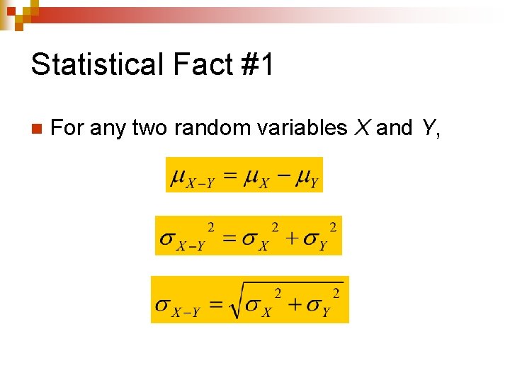
Statistical Fact #1 n For any two random variables X and Y,

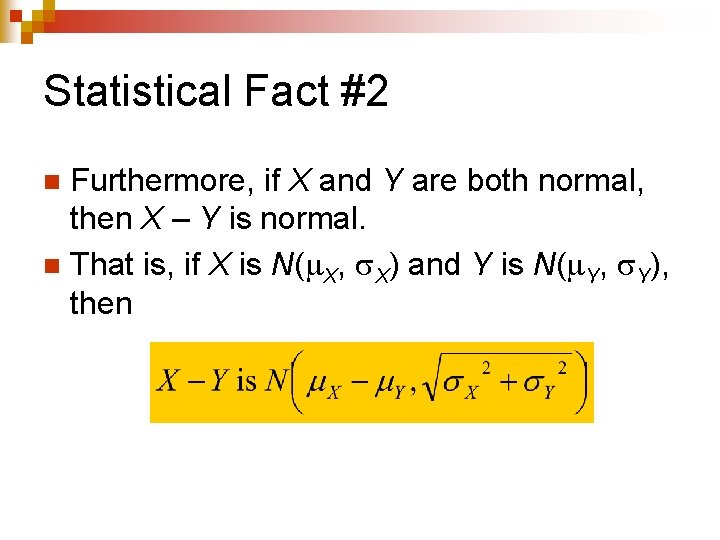
Statistical Fact #2 Furthermore, if X and Y are both normal, then X – Y is normal. n That is, if X is N( X, X) and Y is N( Y, Y), then n

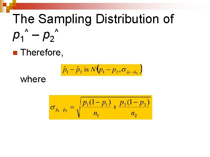
The Sampling Distribution of ^ ^ p 1 – p 2 n Therefore, where

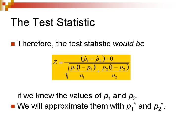
The Test Statistic n Therefore, the test statistic would be if we knew the values of p 1 and p 2. n We will approximate them with p 1^ and p 2^.