Independent Groups 2 The Role of Data Analysis

Independent Groups 2: The Role of Data Analysis in Experiments Methods in Psychological Science Spring 2020 Dr Chapman

Analysis and Interpretation of Experimental Findings • Use statistical analysis to – Claim IV produced an effect on DV – Rule out the alternative explanation that chance produced any observed effect • Replication – Best way to determine whether findings are reliable – Repeat experiment and see if same results are obtained

Analysis of Experimental Designs • Three steps – Check the data • Errors? outliers? – Describe the results • Descriptive statistics such as means, standard deviations, effect size – Confirm what the data reveal • Inferential statistics

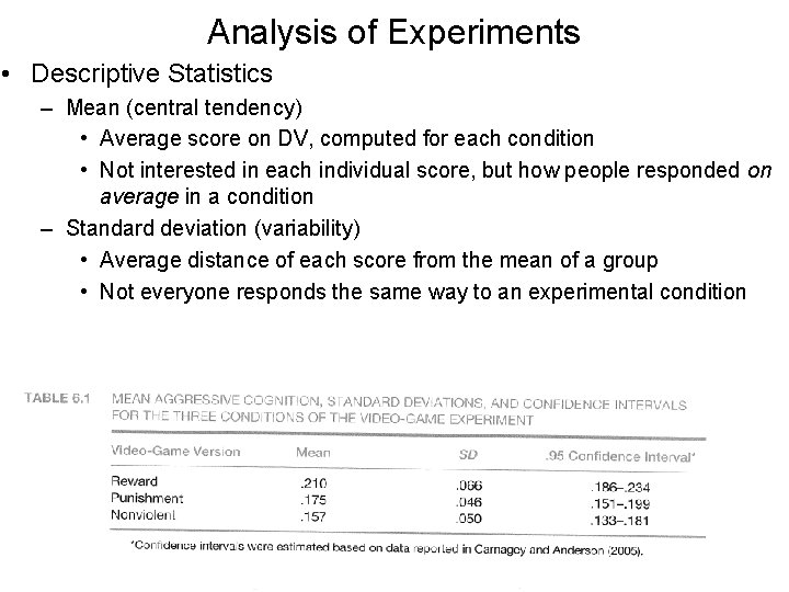
Analysis of Experimental Designs • For example Carnagey and Anderson effects of playing violent video games on aggressive affect, cognition and behavior • I. V. Three versions of video game • Reward condition • Punishment condition • Nonviolent condition • D. V. • Hostile emotions • Aggressive cognition • Aggressive behavior • Procedure • Complete word fragments • Half could be aggressive “K I __ __” • Results • Check for errors • Descriptive statistics

Analysis of Experiments • Descriptive Statistics – Mean (central tendency) • Average score on DV, computed for each condition • Not interested in each individual score, but how people responded on average in a condition – Standard deviation (variability) • Average distance of each score from the mean of a group • Not everyone responds the same way to an experimental condition

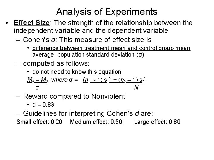
Analysis of Experiments • Effect Size: The strength of the relationship between the independent variable and the dependent variable – Cohen’s d: This measure of effect size is • difference between treatment mean and control group mean average population standard deviation (σ) – computed as follows: • do not need to know this equation M 1 – M 2 where σ = (n 1 - 1) s 12 + (n 2 – 1) s 22 σ N – Reward compared to Nonviolent • d = 0. 83 – Guidelines for interpreting Cohen’s d are: Small effect: 0. 20 Medium effect: 0. 50 Large effect: 0. 80

Analysis of Experiments – Meta-analysis is used to summarize the effect size of an independent variable or dependent variable across many experiments. • Experiments that investigate a psychological phenomenon are selected for review based on their internal validity and other criteria. • An effect size for each experiment is computed (or several effect sizes, depending on the number of variables). • The effect sizes across all the relevant experiments are combined to determine the average effect size across all experiments.

Analysis of Experiments • Confirm what the data reveal – Use inferential statistics to determine whether the IV produced a reliable effect on the DV. – Allow us to rule out whether the findings from our experiment might be simply due to chance (error variation). – Two types of inferential statistics: • Null hypothesis testing • Confidence intervals

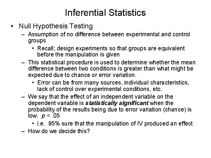
Inferential Statistics • Null Hypothesis Testing – Assumption of no difference between experimental and control groups • Recall; design experiments so that groups are equivalent before the manipulation is given – This statistical procedure is used to determine whether the mean difference between two conditions is greater than what might be expected due to chance or error variation. • Error can be from many sources, individual characteristics, lack of control over experimental conditions, etc. – We say that the effect of an independent variable on the dependent variable is statistically significant when the probability of the results being due to error variation (chance) is low. p <. 05 • i. e. 95% sure that the manipulation of IV produced an effect – How do we decide this?

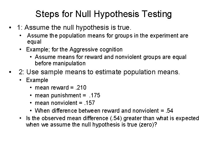
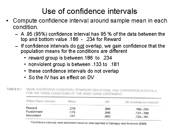
Steps for Null Hypothesis Testing • 1: Assume the null hypothesis is true. • Assume the population means for groups in the experiment are equal • Example; for the Aggressive cognition • Assume means for reward and nonviolent groups are equal before manipulation • 2: Use sample means to estimate population means. • Example • mean reward =. 210 • mean punishment =. 175 • mean nonviolent =. 157 • When difference between reward and nonviolent =. 54 • Is the observed mean difference (. 54) greater than what is expected when we assume the null hypothesis is true (zero)?

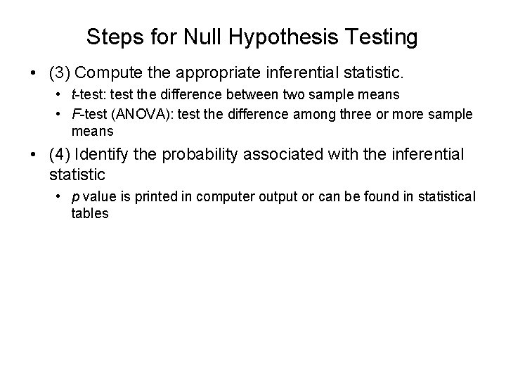
Steps for Null Hypothesis Testing • (3) Compute the appropriate inferential statistic. • t-test: test the difference between two sample means • F-test (ANOVA): test the difference among three or more sample means • (4) Identify the probability associated with the inferential statistic • p value is printed in computer output or can be found in statistical tables

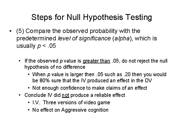
Steps for Null Hypothesis Testing • (5) Compare the observed probability with the predetermined level of significance (alpha), which is usually p <. 05 • If the observed p value is greater than. 05, do not reject the null hypothesis of no difference • When p value is larger then. 05 such as. 20 then you would be 80% sure that the IV produced an effect in the DV • Not enough confidence to make claims of an effect • Conclude IV did not produce a reliable effect • I. V. Three versions of video game • No effect on Aggressive cognition

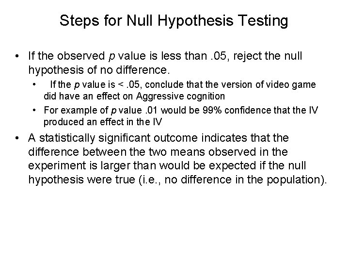
Steps for Null Hypothesis Testing • If the observed p value is less than. 05, reject the null hypothesis of no difference. • If the p value is <. 05, conclude that the version of video game did have an effect on Aggressive cognition • For example of p value. 01 would be 99% confidence that the IV produced an effect in the IV • A statistically significant outcome indicates that the difference between the two means observed in the experiment is larger than would be expected if the null hypothesis were true (i. e. , no difference in the population).

Use of confidence intervals • Compute confidence interval around sample mean in each condition. – A. 95 (95%) confidence interval has 95 % of the data between the top and bottom value. 186 -. 234 for Reward – If confidence intervals do not overlap, we gain confidence that the population means for the conditions are different • reward group is between. 186 to. 234 • nonviolent group is between. 133 to. 181 • these confidence intervals do not overlap • So the IV has an effect on DV

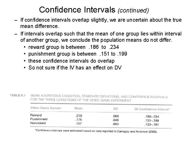
Confidence Intervals (continued) – If confidence intervals overlap slightly, we are uncertain about the true mean difference. – If intervals overlap such that the mean of one group lies within interval of another group, we conclude the population means do not differ. • reward group is between. 186 to. 234 • punishment group is between. 151 to. 199 • these confidence intervals do overlap • So not sure if the IV has an effect on DV

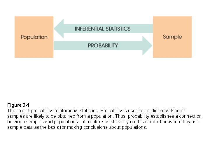
The Role of Probability in Inferential Statistics • Probability is used to predict the type of samples that are likely to be obtained from a population. • Thus, probability establishes a connection between samples and populations. • Inferential statistics rely on this connection when they use sample data as the basis for making conclusions about populations.

Chapter 6 Probability Copyright © 2017 Cengage Learning. All Rights Reserved.

Figure 6 -1 The role of probability in inferential statistics. Probability is used to predict what kind of samples are likely to be obtained from a population. Thus, probability establishes a connection between samples and populations. Inferential statistics rely on this connection when they use sample data as the basis for making conclusions about populations.

Probability • For a situation in which several different outcomes are possible, the probability for any specific outcome is defined as a fraction or a proportion of all the possible outcomes. – If the possible outcomes are identified as A, B, C, D, and so on, then probability of A = number of outcomes classified as A total number of possible outcomes

Probability • Probability is a method for measuring and quantifying the likelihood of obtaining a specific sample from a specific population. • We define probability as a fraction or a proportion. – a ratio comparing the frequency of occurrence for that outcome relative to the total number of possible outcomes. probability of A = number of outcomes classified as Men total number of possible outcomes If there are 12 men and 18 women in a class the probability of picking a man would be 12/30.

Probability and Sampling • To assure that the definition of probability is accurate, the use of random sampling is necessary. – Random sampling requires that each member of a population has an equal chance of being selected. – Independent random sampling includes the conditions of random sampling and further requires that the probability of being selected remains constant for each selection. Also called sampling with replacement. • Because sampling is picking an available person from a population once that person is included in the sample they are no longer available. Need to replace that person before picking the next person so that the probability remains constant.

Probability and Frequency Distributions • The situations in which we are concerned with probability usually involve a population of scores that can be displayed in a frequency distribution graph. • If you think of the graph as representing the entire population, then different portions of the graph represent different portions of the population. • Because probabilities and proportions are equivalent, a particular portion of the graph corresponds to a particular probability.

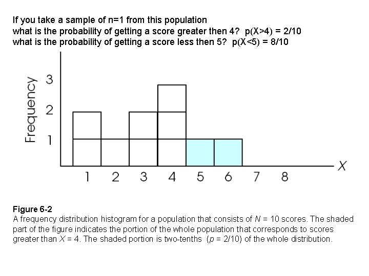
If you take a sample of n=1 from this population what is the probability of getting a score greater then 4? p(X>4) = 2/10 what is the probability of getting a score less then 5? p(X<5) = 8/10 Figure 6 -2 A frequency distribution histogram for a population that consists of N = 10 scores. The shaded part of the figure indicates the portion of the whole population that corresponds to scores greater than X = 4. The shaded portion is two-tenths (p = 2/10) of the whole distribution.

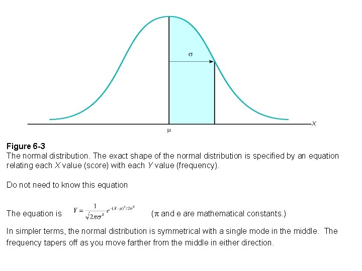
Probability and the Normal Distribution • If a vertical line is drawn through a normal distribution, several things occur. – The line divides the distribution into two sections. The larger section is called the body and the smaller section is called the tail. – The exact location of the line can be specified by a z-score.

Figure 6 -3 The normal distribution. The exact shape of the normal distribution is specified by an equation relating each X value (score) with each Y value (frequency). Do not need to know this equation The equation is ( and e are mathematical constants. ) In simpler terms, the normal distribution is symmetrical with a single mode in the middle. The frequency tapers off as you move farther from the middle in either direction.

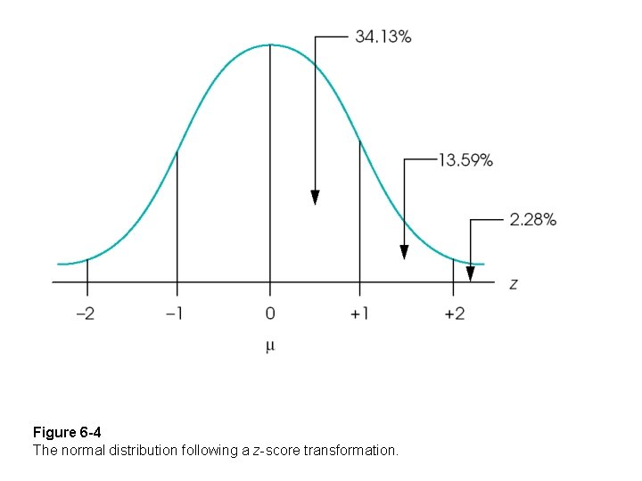
Figure 6 -4 The normal distribution following a z-score transformation.

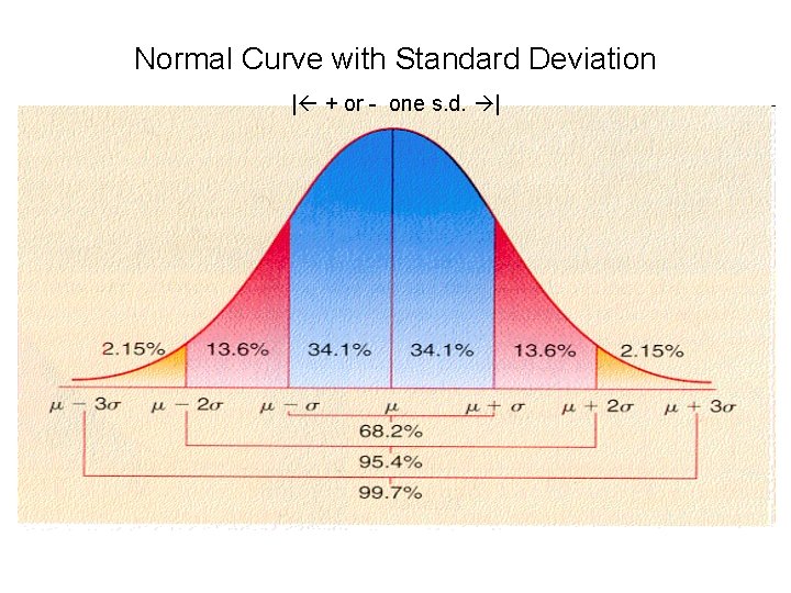
Normal Curve with Standard Deviation | + or - one s. d. |

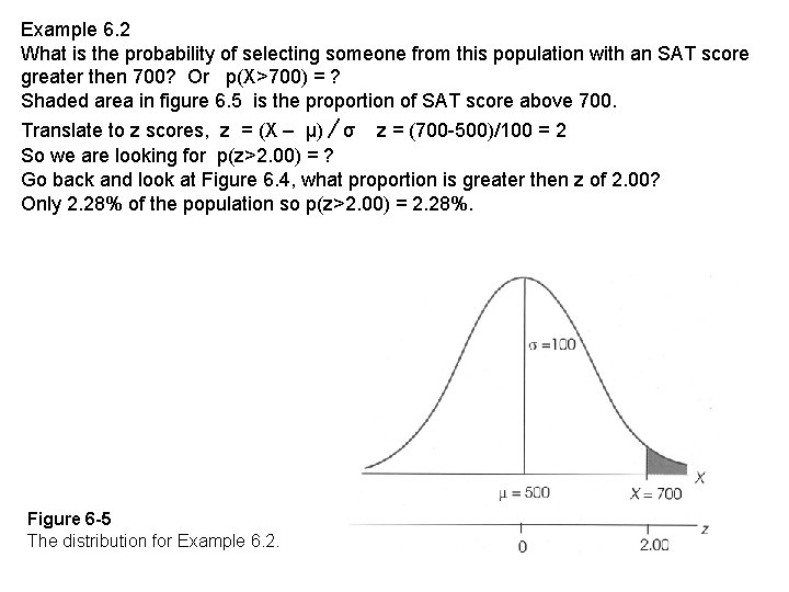
Example 6. 2 What is the probability of selecting someone from this population with an SAT score greater then 700? Or p(X>700) = ? Shaded area in figure 6. 5 is the proportion of SAT score above 700. Translate to z scores, z = (X – μ) ∕ σ z = (700 -500)/100 = 2 So we are looking for p(z>2. 00) = ? Go back and look at Figure 6. 4, what proportion is greater then z of 2. 00? Only 2. 28% of the population so p(z>2. 00) = 2. 28%. Figure 6 -5 The distribution for Example 6. 2.

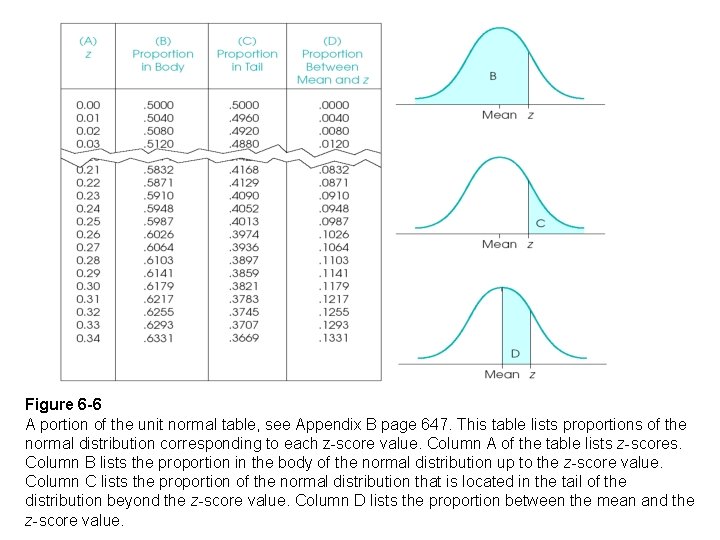
Probability and the Normal Distribution • The unit normal table lists several different proportions corresponding to each z-score location. – Column A of the table lists z-score values. – For each z-score location, columns B and C list the proportions in the body and tail, respectively. – Finally, column D lists the proportion between the mean and the z-score location. • Because probability is equivalent to proportion, the table values can also be used to determine probabilities.

Figure 6 -6 A portion of the unit normal table, see Appendix B page 647. This table lists proportions of the normal distribution corresponding to each z-score value. Column A of the table lists z-scores. Column B lists the proportion in the body of the normal distribution up to the z-score value. Column C lists the proportion of the normal distribution that is located in the tail of the distribution beyond the z-score value. Column D lists the proportion between the mean and the z-score value.

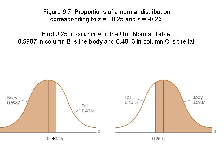
Figure 6. 7 Proportions of a normal distribution corresponding to z = +0. 25 and z = -0. 25. Find 0. 25 in column A in the Unit Normal Table. 0. 5987 in column B is the body and 0. 4013 in column C is the tail +

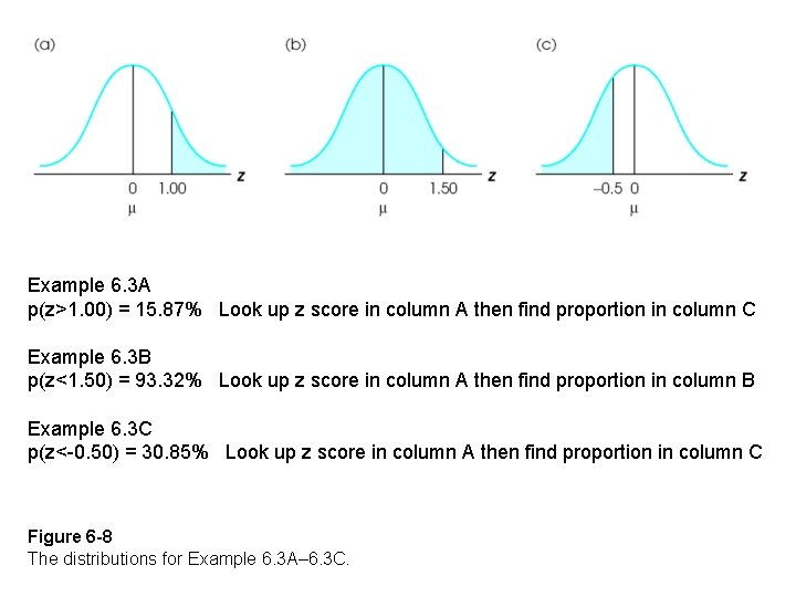
Example 6. 3 A p(z>1. 00) = 15. 87% Look up z score in column A then find proportion in column C Example 6. 3 B p(z<1. 50) = 93. 32% Look up z score in column A then find proportion in column B Example 6. 3 C p(z<-0. 50) = 30. 85% Look up z score in column A then find proportion in column C Figure 6 -8 The distributions for Example 6. 3 A– 6. 3 C.

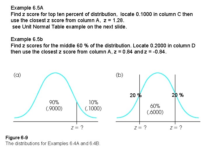
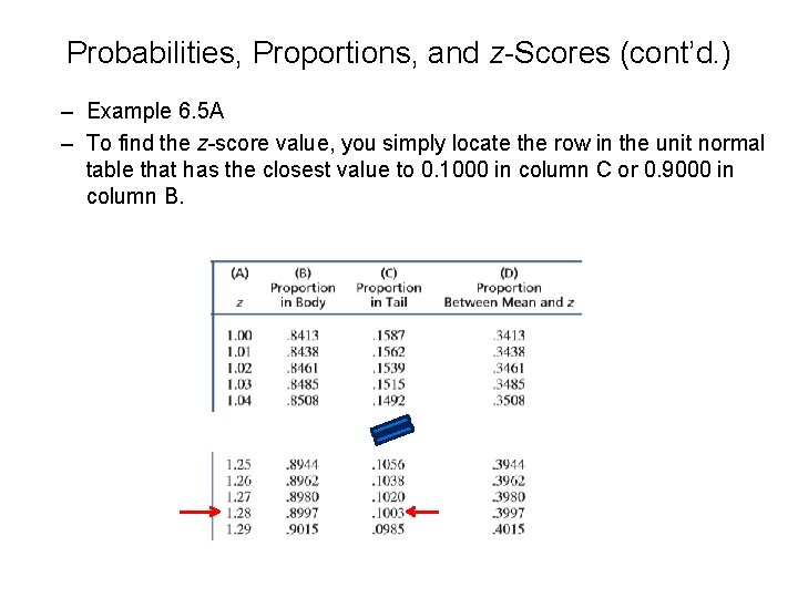
Example 6. 5 A Find z score for top ten percent of distribution, locate 0. 1000 in column C then use the closest z score from column A, z = 1. 28. see Unit Normal Table example on the next slide. Example 6. 5 b Find z scores for the middle 60 % of the distribution. Locate 0. 2000 in column D then use the closest z score from column A, z = 0. 84 and z = -0. 84. 20 % Figure 6 -9 The distributions for Examples 6. 4 A and 6. 4 B. 20 %

Probabilities, Proportions, and z-Scores (cont’d. ) – Example 6. 5 A – To find the z-score value, you simply locate the row in the unit normal table that has the closest value to 0. 1000 in column C or 0. 9000 in column B.