Incorporating uncertainty in distancematrix phylogenetics Wally Gilks Tom
- Slides: 14

Incorporating uncertainty in distance-matrix phylogenetics Wally Gilks Tom Nye Pietro Liò Leeds University Newcastle University Cambridge University Isaac Newton Institute December 17, 2007

Distance-based methods • Larger trees • Faster algorithms • Less model-dependent – Genome-scale evolutionary rearrangements

Agglomerative distance methods • NJ (Saitou and Nei, 1987) • Bio. NJ (Gascuel, 1997) • Weighbor (Bruno et al, 2000) • MVR (Gascuel, 2000) • Fast. ME (Desper and Gascuel, 2004)

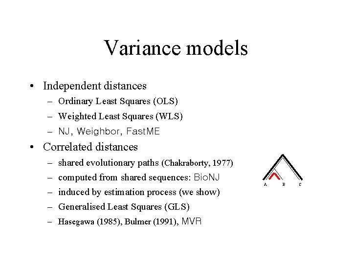
Variance models • Independent distances – Ordinary Least Squares (OLS) – Weighted Least Squares (WLS) A – NJ, Weighbor, Fast. ME • Correlated distances – – shared evolutionary paths (Chakraborty, 1977) computed from shared sequences: Bio. NJ induced by estimation process (we show) Generalised Least Squares (GLS) – Hasegawa (1985), Bulmer (1991), MVR A B C

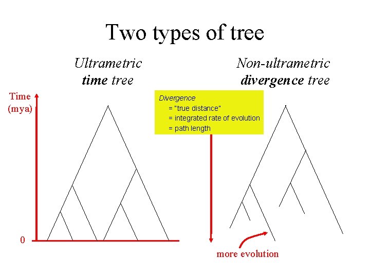
Two types of tree Ultrametric time tree Time (mya) Non-ultrametric divergence tree Divergence = “true distance” = integrated rate of evolution = path length 0 more evolution

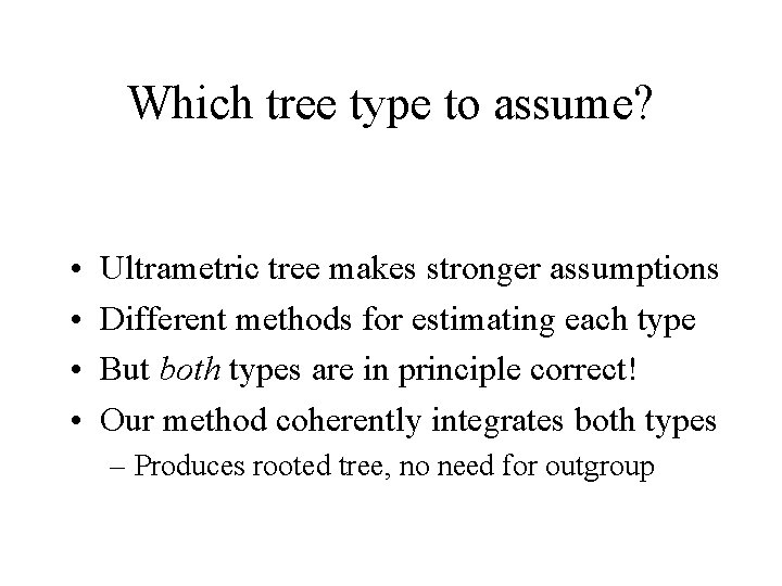
Which tree type to assume? • • Ultrametric tree makes stronger assumptions Different methods for estimating each type But both types are in principle correct! Our method coherently integrates both types – Produces rooted tree, no need for outgroup

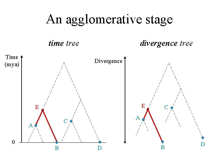
An agglomerative stage time tree Time (mya) divergence tree Divergence E E 0 A C A B C D B D

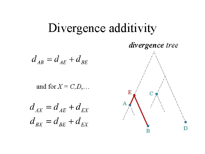
Divergence additivity divergence tree and for X = C, D, … E C A B D

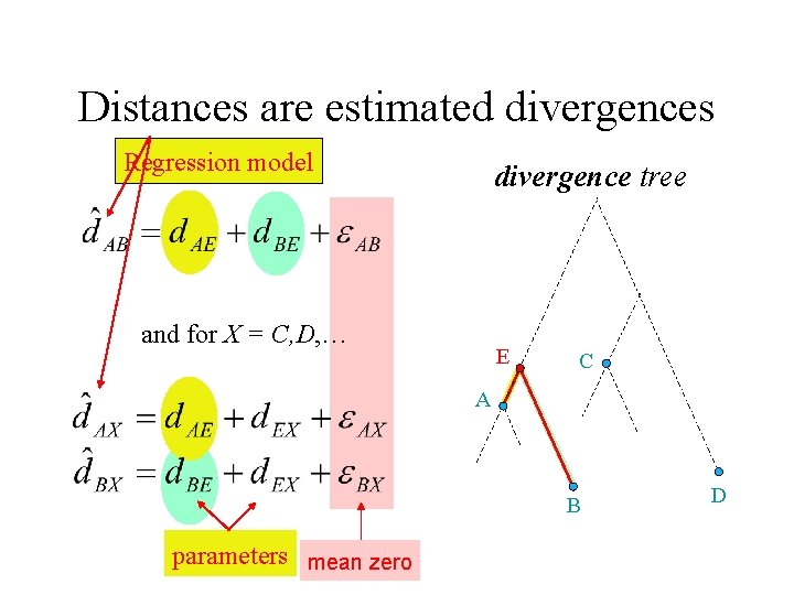
Distances are estimated divergences Regression model divergence tree and for X = C, D, … E C A B parameters mean zero D

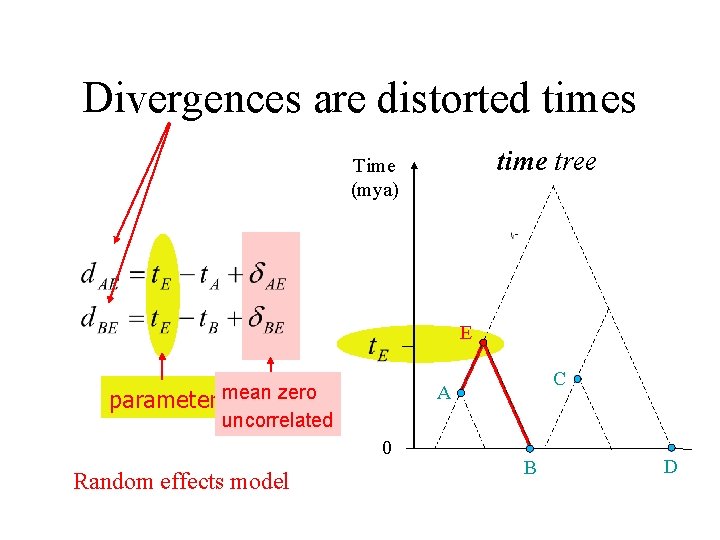
Divergences are distorted times time tree Time (mya) E parameter mean zero uncorrelated 0 Random effects model C A B D

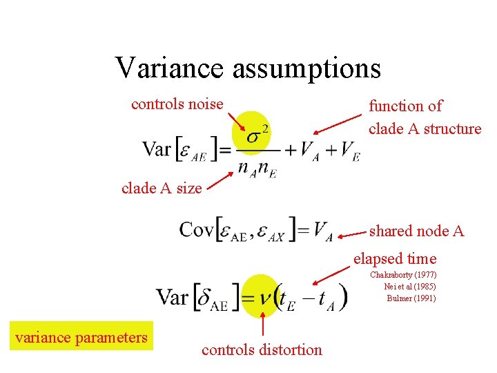
Variance assumptions controls noise function of clade A structure clade A size shared node A elapsed time Chakraborty (1977) Nei et al (1985) Bulmer (1991) variance parameters controls distortion

Estimation • Time tree and divergence tree are estimated simultaneously – by GLS (Hasegawa, 1985; Bulmer, 1991) • Choose most recent agglomeration always • Estimated divergences become the distances for the next stage – Variance formula accommodates estimation-induced correlations

Notes • Can estimate variance parameters s 2 and n • Computationally efficient algorithm – same time-complexity as Bio. NJ – we call it Stat. Tree

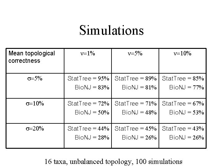
Simulations Mean topological correctness n=1% n=5% n=10% s=5% Stat. Tree = 95% Stat. Tree = 89% Stat. Tree = 85% Bio. NJ = 83% Bio. NJ = 81% Bio. NJ = 77% s=10% Stat. Tree = 72% Stat. Tree = 71% Stat. Tree = 67% Bio. NJ = 50% Bio. NJ = 48% Bio. NJ = 53% s=20% Stat. Tree = 44% Stat. Tree = 45% Stat. Tree = 43% Bio. NJ = 28% Bio. NJ = 26% 16 taxa, unbalanced topology, 100 simulations