Income Determination The Monetary Dimension II Overview Keynesian

Income Determination The Monetary Dimension - II

Overview $ Keynesian Income Determination Models Private sector Consumption demand Investment Demand Supply & demand for money Public Sector Government expenditure Government taxes Monetary policy manipulation of money supply International imports, exports, net exports

Money Demand $ In Classical economics we saw an analysis of the supply and demand for "loanable funds" supply = deposits in banks of money being saved demand = borrowing from banks deposits, mostly for investment $ In Keynesian analysis focus shifts to demand for money, to those who want to hold money, as opposed to interest bearing assets and their reasons

Keynes gave three motives $ Transactions demand $ Precautionary demand $ Speculative demand

Cost of holding money $ Money vs C&F's "bond" $ If you hold cash, you earn no interest income $ If you hold an interest bearing account you do earn interest $ So, assuming profit maximizing behavior, you would expect people to deposit all their money into interest bearing assets unless they had reasons to do otherwise

Transaction Demand $ Main reason to hold money: to have it on hand to finance various transactions you keep money in your pocket to by a coke you keep money in your checking acct to pay rent businesses keep money for regular purchases $ Income and transaction demand income and spending are not synchronized e. g. , incomes in once a month e. g. , money needs to be spent more frequently

Optimal Balance $ On the one hand you want to earn interest $ On the other you need money in hand $ How much?

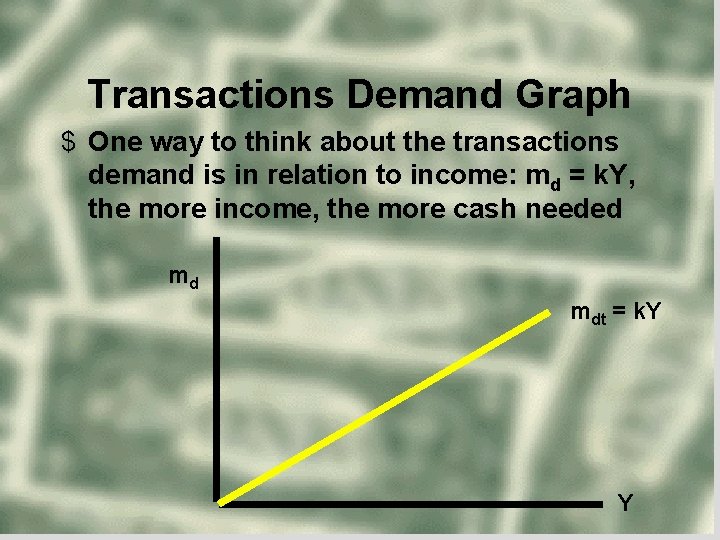
Transactions Demand Graph $ One way to think about the transactions demand is in relation to income: md = k. Y, the more income, the more cash needed md mdt = k. Y Y

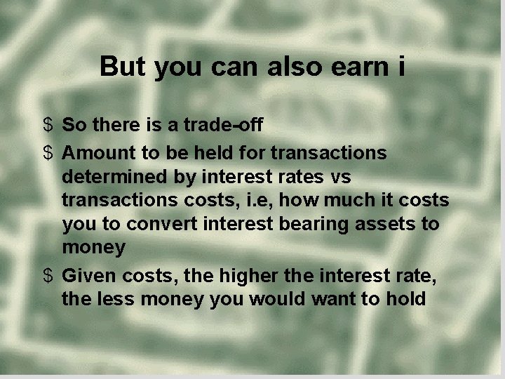
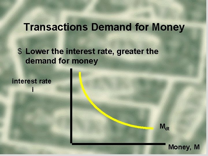
But you can also earn i $ So there is a trade-off $ Amount to be held for transactions determined by interest rates vs transactions costs, i. e, how much it costs you to convert interest bearing assets to money $ Given costs, the higher the interest rate, the less money you would want to hold

Transactions Demand for Money $ Lower the interest rate, greater the demand for money interest rate i Mdt Money, M

Precautionary Demand $ People hold money because they can't anticipate every need, there is uncertainty, so they hold more $ With uncertainty independent of the interest rate then you might expect the Md curve to be a little more to the right than otherwise. $ "IF" the interest rate measures risk, then the Md curve might be steeper

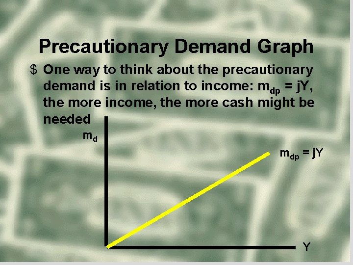
Precautionary Demand Graph $ One way to think about the precautionary demand is in relation to income: mdp = j. Y, the more income, the more cash might be needed md mdp = j. Y Y

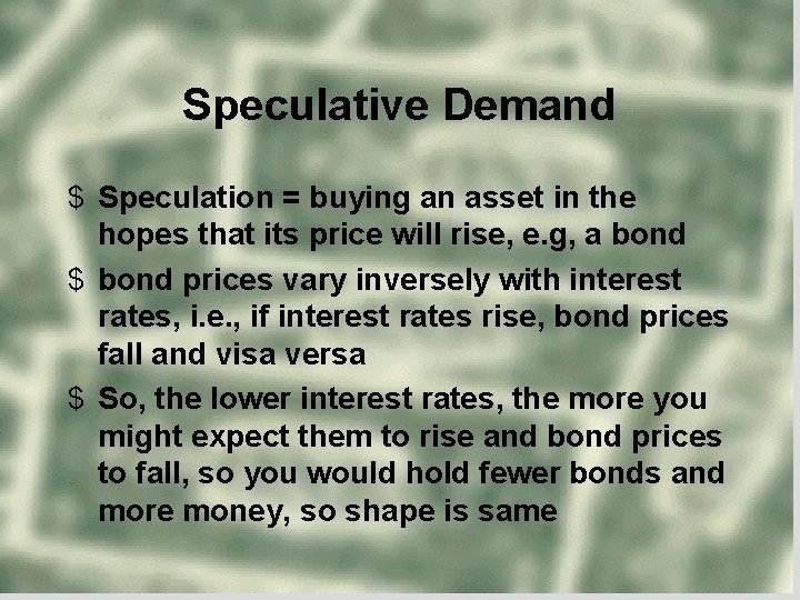
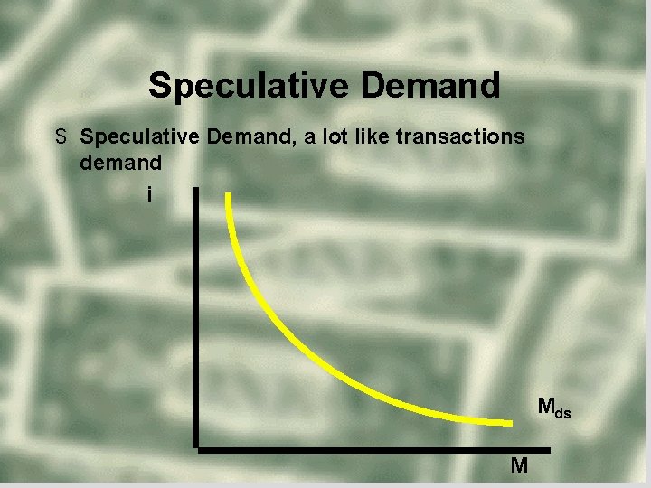
Speculative Demand $ Speculation = buying an asset in the hopes that its price will rise, e. g, a bond $ bond prices vary inversely with interest rates, i. e. , if interest rates rise, bond prices fall and visa versa $ So, the lower interest rates, the more you might expect them to rise and bond prices to fall, so you would hold fewer bonds and more money, so shape is same

Speculative Demand $ Speculative Demand, a lot like transactions demand i Mds M

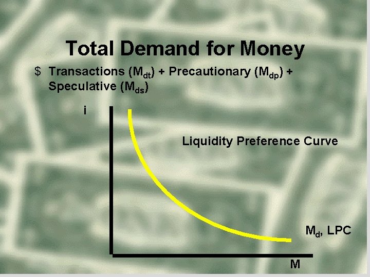
Total Demand for Money $ Transactions (Mdt) + Precautionary (Mdp) + Speculative (Mds) i Liquidity Preference Curve Md, LPC M

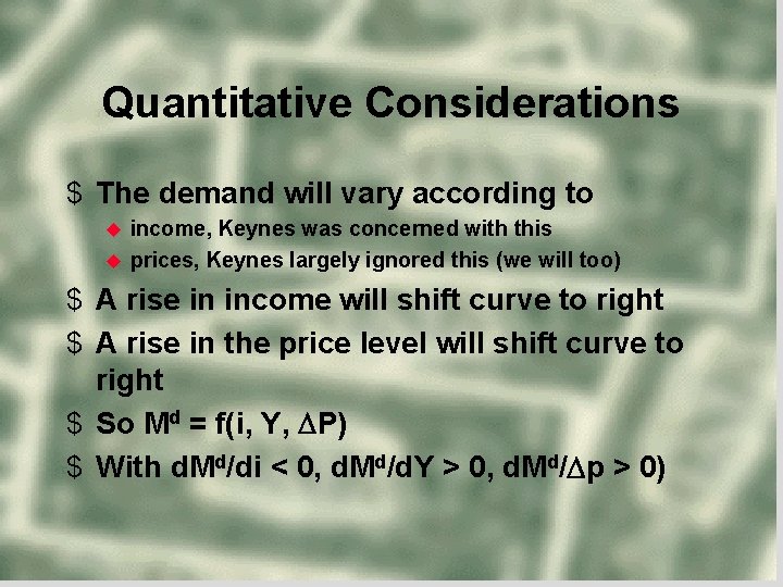
Quantitative Considerations $ The demand will vary according to income, Keynes was concerned with this prices, Keynes largely ignored this (we will too) $ A rise in income will shift curve to right $ A rise in the price level will shift curve to right $ So Md = f(i, Y, P) $ With d. Md/di < 0, d. Md/d. Y > 0, d. Md/ p > 0)

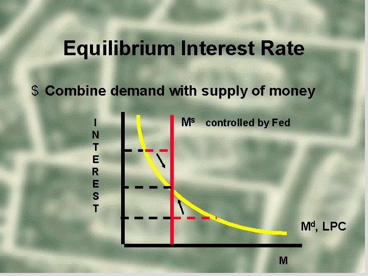
Equilibrium Interest Rate $ Combine demand with supply of money I N T E R E S T Ms controlled by Fed Md, LPC M

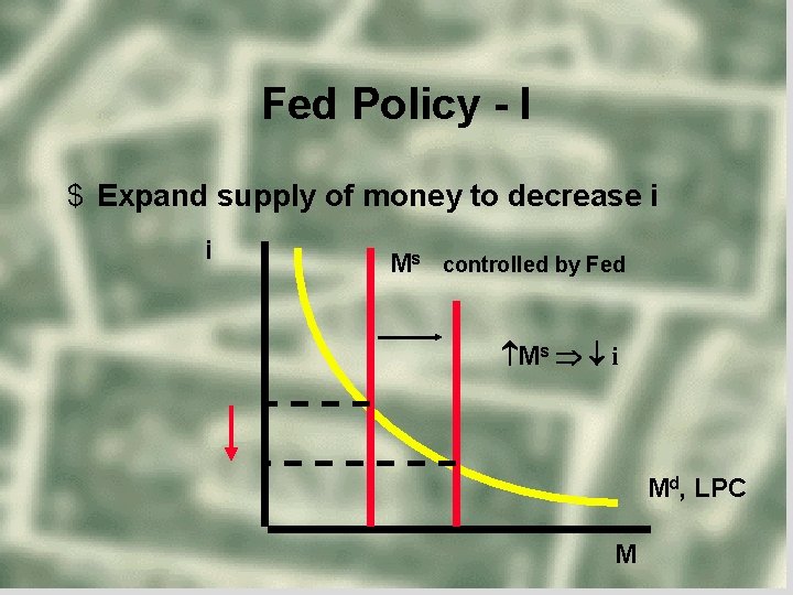
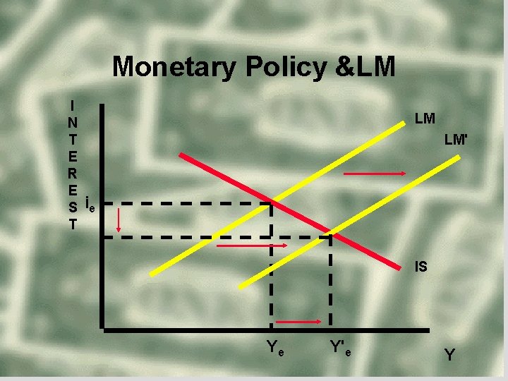
Fed Policy - I $ Expand supply of money to decrease i i Ms controlled by Fed Ms i Md, LPC M

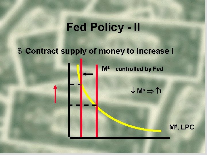
Fed Policy - II $ Contract supply of money to increase i Ms controlled by Fed Ms i Md, LPC

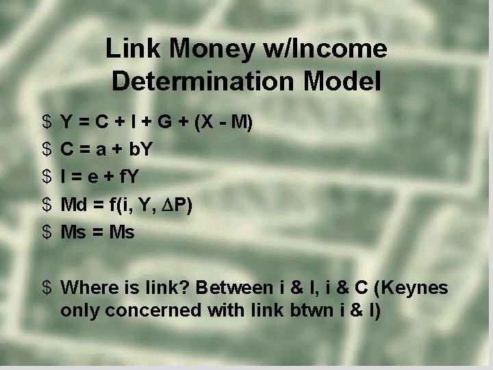
Link Money w/Income Determination Model $ $ $ Y = C + I + G + (X - M) C = a + b. Y I = e + f. Y Md = f(i, Y, P) Ms = Ms $ Where is link? Between i & I, i & C (Keynes only concerned with link btwn i & I)

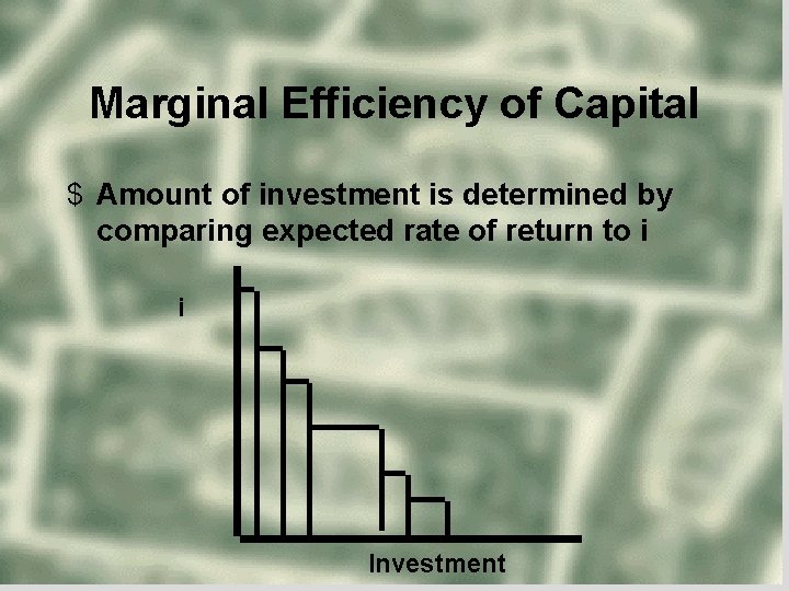
Marginal Efficiency of Capital $ Amount of investment is determined by comparing expected rate of return to i i Investment

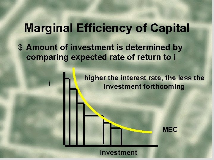
Marginal Efficiency of Capital $ Amount of investment is determined by comparing expected rate of return to i i higher the interest rate, the less the investment forthcoming MEC Investment

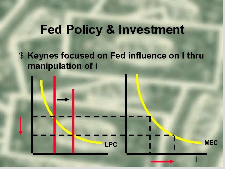
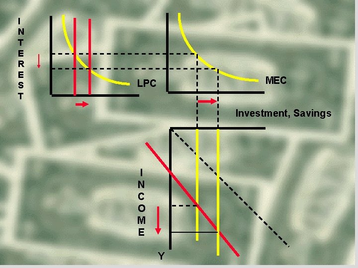
Fed Policy & Investment $ Keynes focused on Fed influence on I thru manipulation of i MEC LPC I

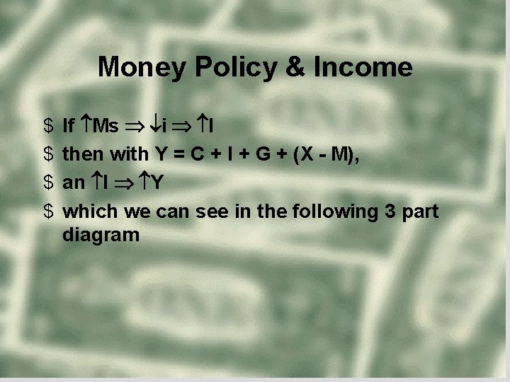
Money Policy & Income $ $ If Ms i I then with Y = C + I + G + (X - M), an I Y which we can see in the following 3 part diagram

I N T E R E S T MEC LPC Investment, Savings I N C O M E Y

Feedback Effect $ However, remembering that $ Md = f(i, Y, P), d. Md/d. Y > 0 $ We know that an increase in Y will result in a right shift in Md, offsetting the increase in Ms somewhat so i won't be quite as low, and thus also I & Y won't increase as much $ Two solutions: algebraic change models

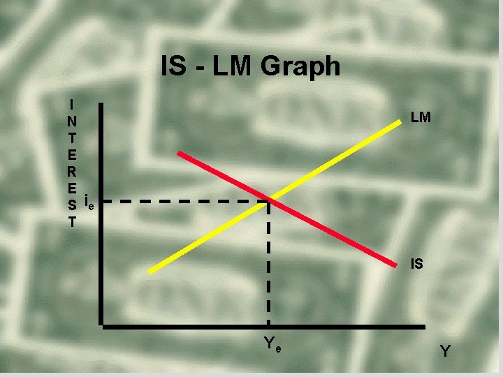
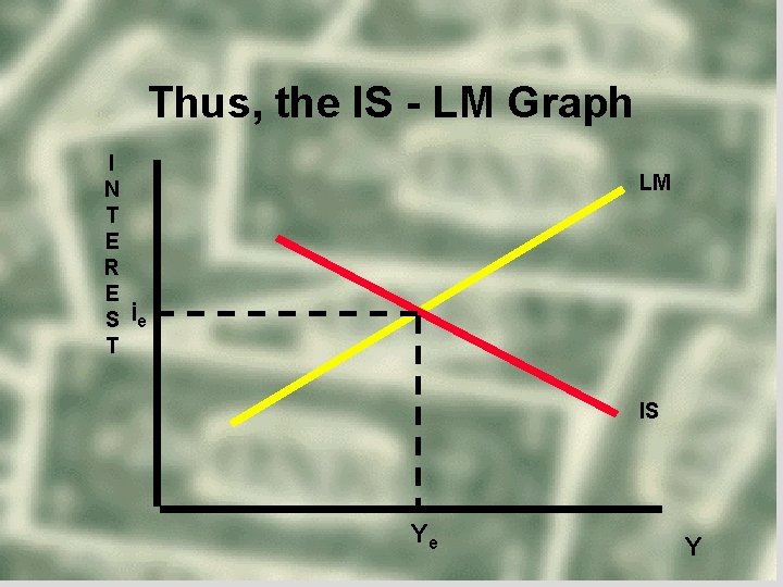
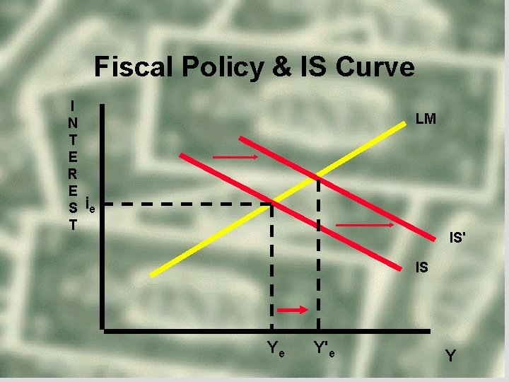
IS - LM Model $ Alternative formulation of Keynesian model which moves consumption to background and highlights interest rate. $ IS = locus of equilibrium points between investment and supply (I & S, IS) $ LM = locus of equilibrium points in supply & demand for money.

IS - LM Graph I N T E R E S T LM ie IS Ye Y

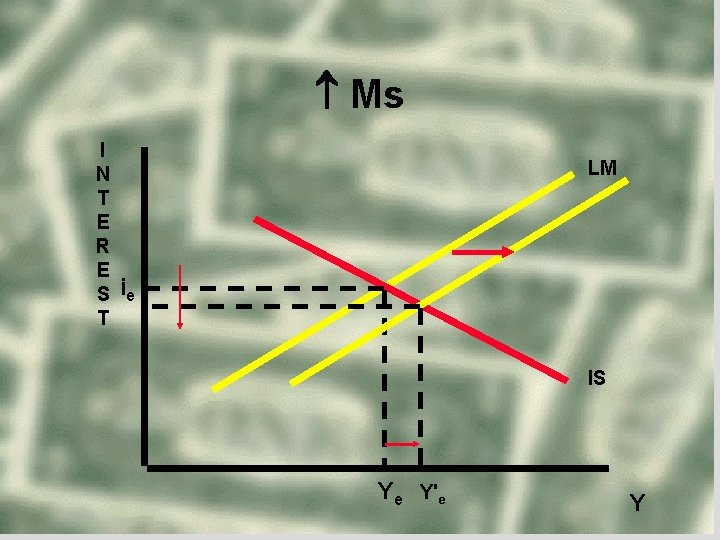
Ms I N T E R E S T LM ie IS Ye Y'e Y

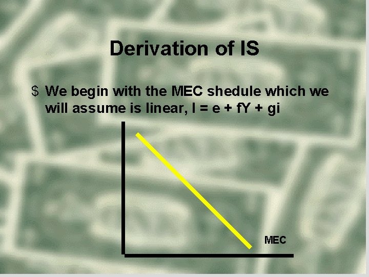
Derivation of IS $ We begin with the MEC shedule which we will assume is linear, I = e + f. Y + gi MEC

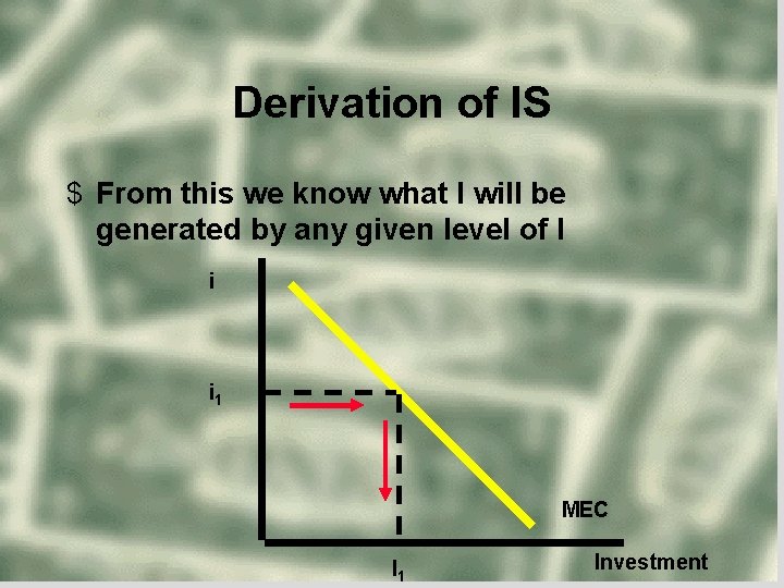
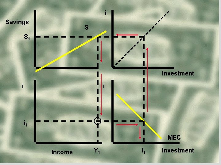
Derivation of IS $ From this we know what I will be generated by any given level of I i i 1 MEC I 1 Investment

Algebraic $ If our linear MEC curve is given by the equation I = e +gi, [or i = e + g. I] w/g<0 NB: given our past discussion of investment we would be more likely to use I = e + f. Y +gi. This would cause no problem in solving the model for equilibrium Y, but in this simple graphic derivation we leave Y out because it is Y we are looking for. ) $ Then for any given i we can calculate the level of investment, I that we would expect to be forthcoming at that I.

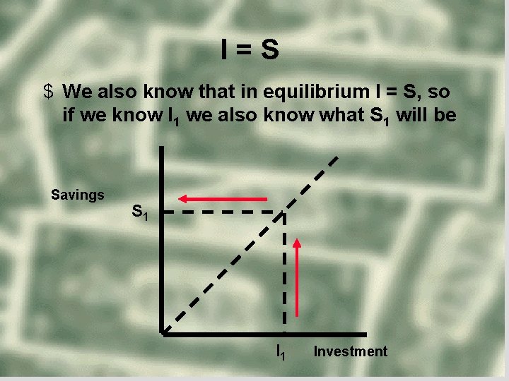
I=S $ We also know that in equilibrium I = S, so if we know I 1 we also know what S 1 will be Savings S 1 Investment

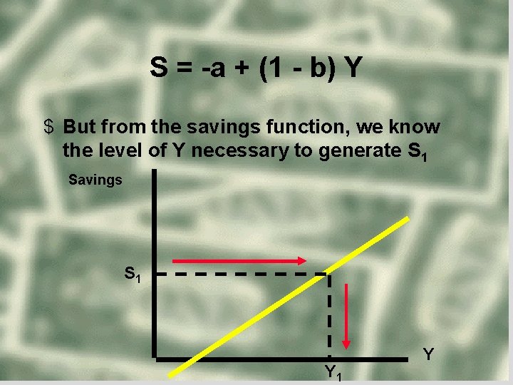
S = -a + (1 - b) Y $ But from the savings function, we know the level of Y necessary to generate S 1 Savings S 1 Y

Algebraic $ Given a rate of interest (i), we found the resulting level of investment (I) $ We know that in equilibrium, I = S $ Therefore, we know S $ The only question that remains is what level of Y will generate that level of S $ We can find this from the Savings function (S = -a + (1 -b)Y)

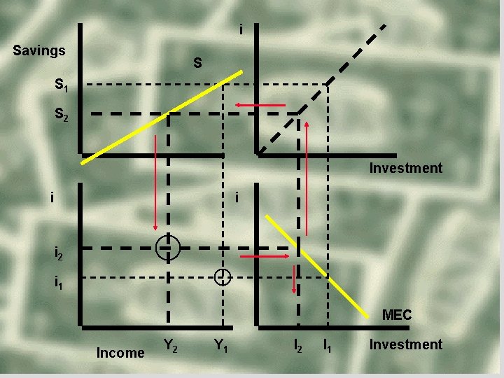
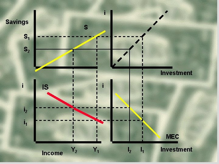
Equilibrium Point $ So, beginning with a given interest rate, we have found the level of Y at which I = S. $ We can repeat this procedure to obtain the locus of points that forms the IS curve. $ We can also put these four diagrams together to see their interaction

i Savings S S 1 Investment i i i 1 MEC Income Y 1 Investment

i Savings S S 1 S 2 Investment i i i 2 i 1 MEC Income Y 2 Y 1 I 2 I 1 Investment

i Savings S S 1 S 2 Investment i i IS i 2 i 1 MEC Income Y 2 Y 1 I 2 I 1 Investment

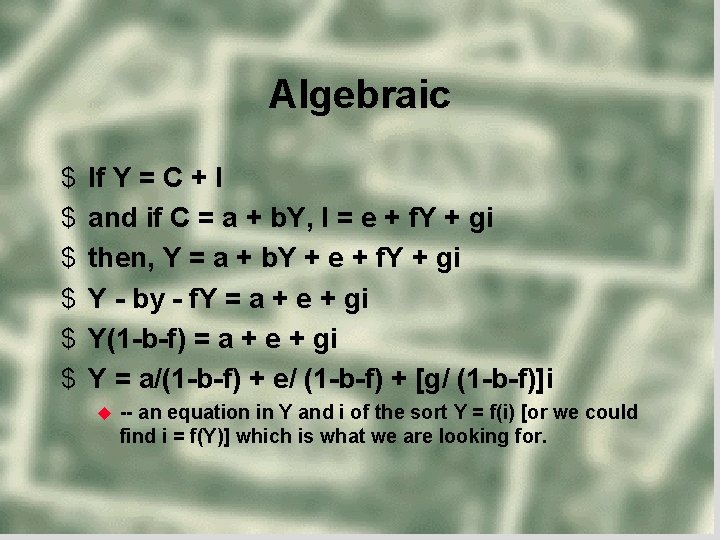
Algebraic $ $ $ If Y = C + I and if C = a + b. Y, I = e + f. Y + gi then, Y = a + b. Y + e + f. Y + gi Y - by - f. Y = a + e + gi Y(1 -b-f) = a + e + gi Y = a/(1 -b-f) + e/ (1 -b-f) + [g/ (1 -b-f)]i -- an equation in Y and i of the sort Y = f(i) [or we could find i = f(Y)] which is what we are looking for.

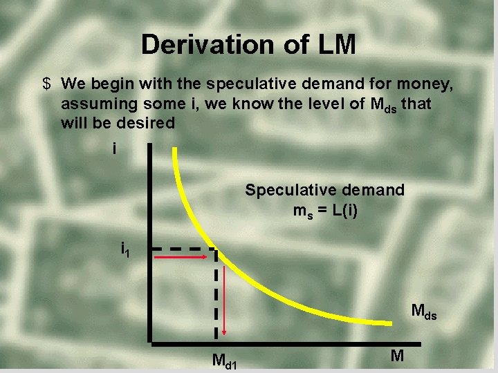
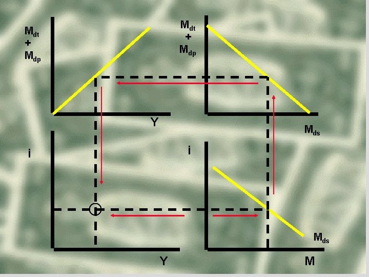
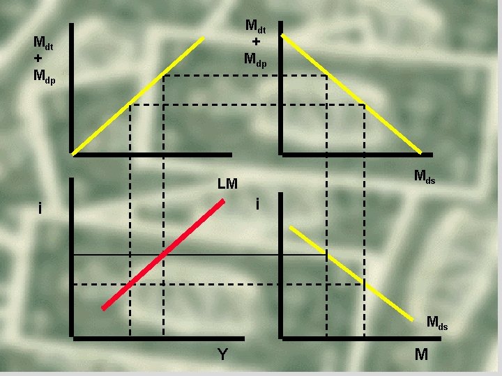
Derivation of LM $ We begin with the speculative demand for money, assuming some i, we know the level of Mds that will be desired i Speculative demand ms = L(i) i 1 Mds Md 1 M

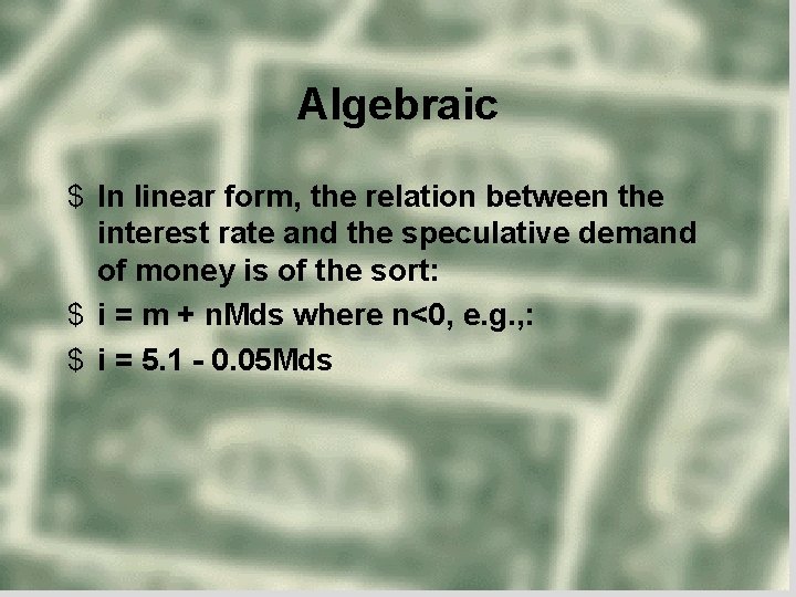
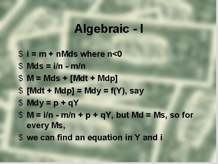
Algebraic $ In linear form, the relation between the interest rate and the speculative demand of money is of the sort: $ i = m + n. Mds where n<0, e. g. , : $ i = 5. 1 - 0. 05 Mds

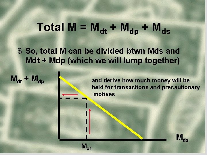
Total M = Mdt + Mdp + Mds $ So, total M can be divided btwn Mds and Mdt + Mdp (which we will lump together) Mdt + Mdp and derive how much money will be held for transactions and precautionary motives Md 1 Mds

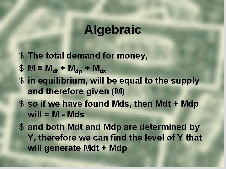
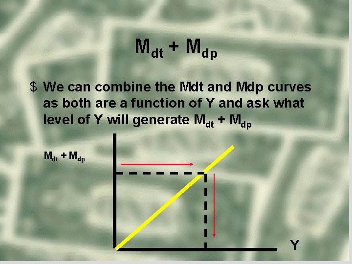
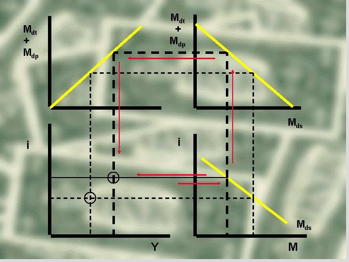
Algebraic $ The total demand for money, $ M = Mdt + Mdp + Mds $ in equilibrium, will be equal to the supply and therefore given (M) $ so if we have found Mds, then Mdt + Mdp will = M - Mds $ and both Mdt and Mdp are determined by Y, therefore we can find the level of Y that will generate Mdt + Mdp

Mdt + Mdp $ We can combine the Mdt and Mdp curves as both are a function of Y and ask what level of Y will generate Mdt + Mdp Y

One Point on LM $ We now have a level of Y that will be compatible with the originally posited level of interest. That level of Y will generate a level of transactions and precautionary demand compatible with the desired level of speculative demand. $ We can see the relationships in the following diagram.

Mdt + Mdp Y Mds i i Mds Y M

Mdt + Mdp Mds i i Mds Y M

Mdt + Mdp Mds LM i i Mds Y M

Algebraic - I $ $ $ i = m + n. Mds where n<0 Mds = i/n - m/n M = Mds + [Mdt + Mdp] = Mdy = f(Y), say Mdy = p + q. Y M = i/n - m/n + p + q. Y, but Md = Ms, so for every Ms, $ we can find an equation in Y and i

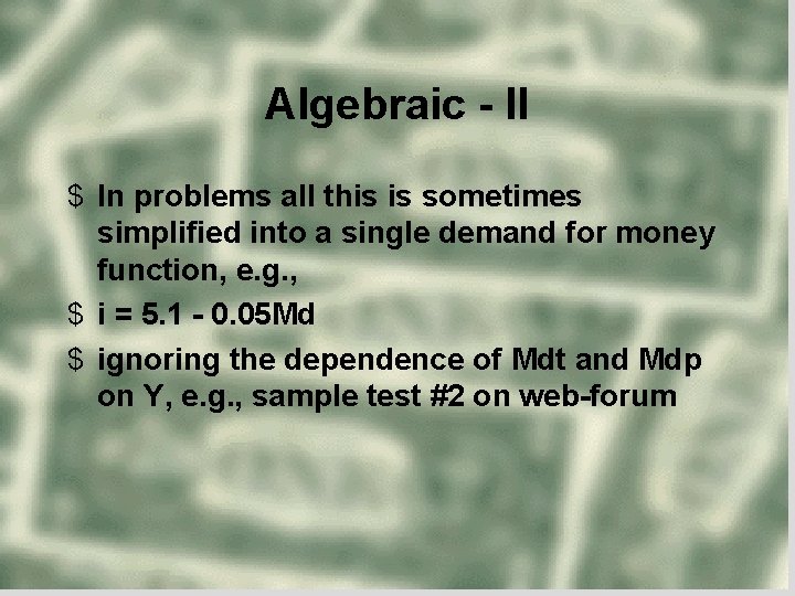
Algebraic - II $ In problems all this is sometimes simplified into a single demand for money function, e. g. , $ i = 5. 1 - 0. 05 Md $ ignoring the dependence of Mdt and Mdp on Y, e. g. , sample test #2 on web-forum

Thus, the IS - LM Graph I N T E R E S T LM ie IS Ye Y

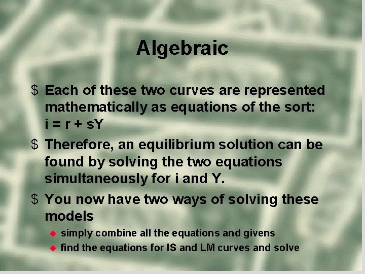
Algebraic $ Each of these two curves are represented mathematically as equations of the sort: i = r + s. Y $ Therefore, an equilibrium solution can be found by solving the two equations simultaneously for i and Y. $ You now have two ways of solving these models simply combine all the equations and givens find the equations for IS and LM curves and solve

Fiscal Policy & IS Curve I N T E R E S T LM ie IS' IS Ye Y'e Y

Monetary Policy &LM I N T E R E S T LM LM' ie IS Ye Y'e Y

Homework $ Now, factor in G and T and re-derive the IS and LM curves. How does their inclusion change the graphs? $ Finally, factor in net exports (X - M) and do the same.

--END--