Income and Spending Chapter 10 AD and Equilibrium
Income and Spending Chapter #10
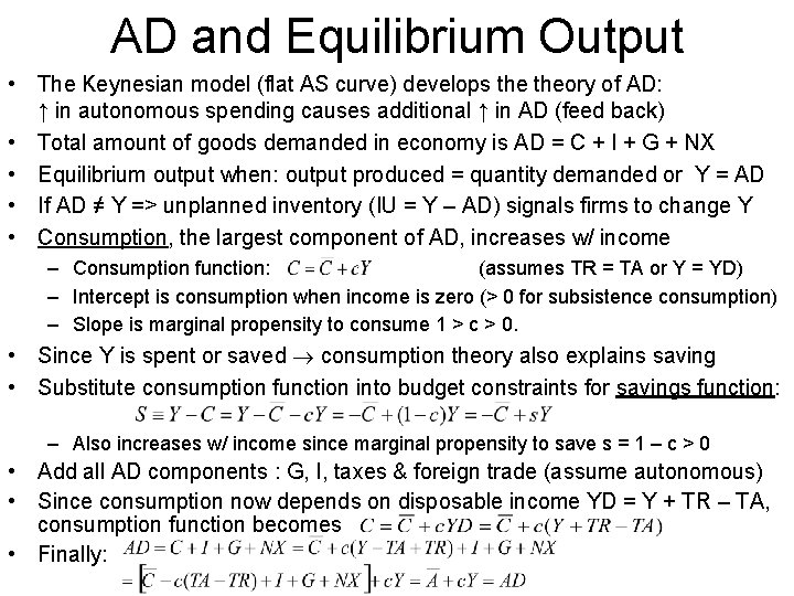
AD and Equilibrium Output • The Keynesian model (flat AS curve) develops theory of AD: ↑ in autonomous spending causes additional ↑ in AD (feed back) • Total amount of goods demanded in economy is AD = C + I + G + NX • Equilibrium output when: output produced = quantity demanded or Y = AD • If AD ≠ Y => unplanned inventory (IU = Y – AD) signals firms to change Y • Consumption, the largest component of AD, increases w/ income – Consumption function: (assumes TR = TA or Y = YD) – Intercept is consumption when income is zero (> 0 for subsistence consumption) – Slope is marginal propensity to consume 1 > c > 0. • Since Y is spent or saved consumption theory also explains saving • Substitute consumption function into budget constraints for savings function: – Also increases w/ income since marginal propensity to save s = 1 – c > 0 • Add all AD components : G, I, taxes & foreign trade (assume autonomous) • Since consumption now depends on disposable income YD = Y + TR – TA, consumption function becomes • Finally:
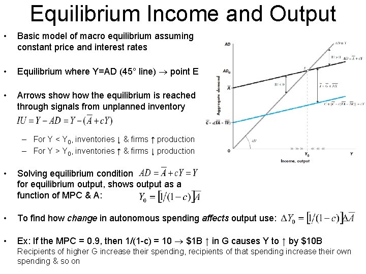
Equilibrium Income and Output • Basic model of macro equilibrium assuming constant price and interest rates • Equilibrium where Y=AD (45° line) point E • Arrows show the equilibrium is reached through signals from unplanned inventory – For Y < Y 0, inventories ↓ & firms ↑ production – For Y > Y 0, inventories ↑ & firms ↓ production • Solving equilibrium condition for equilibrium output, shows output as a function of MPC & A: • To find how change in autonomous spending affects output use: • Ex: If the MPC = 0. 9, then 1/(1 -c) = 10 $1 B ↑ in G causes Y to ↑ by $10 B Recipients of higher G increase their spending, recipients of that spending increase their own spending & so on
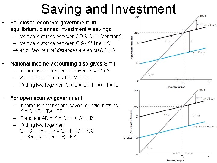
Saving and Investment • For closed econ w/o government, in equilibrium, planned investment = savings – Vertical distance between AD & C = I (constant) – Vertical distance between C & 45° line = S at Y 0 two vertical distances are equal & I = S • National income accounting also gives S = I – Income is either spent or saved: Y = C + S – Without G or trade: AD = Y = C + I – Putting two together: C + S = C + I => I = S • For open econ w/ government: – Income is either spent, saved, or paid in taxes: Y = C + S + TA - TR – Complete AD = Y = C + I + G + NX – Putting two together: C + S + TA – TR = C + I + G + NX I = S + (TA – TR – G) - NX
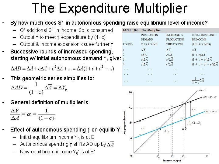
The Expenditure Multiplier • By how much does $1 in autonomous spending raise equilibrium level of income? – Of additional $1 in income, $c is consumed – Output ↑ to meet ↑ expenditure by (1+c) – Output & income expansion cause further ↑ • Successive rounds of increased spending, starting w/ initial autonomous demand ↑, give: (15) • This geometric series simplifies to: • General definition of multiplier is • Effect of autonomous spending ↑ on equilib Y: – Initial equilibrium income Y 0 is at E – Autonomous spending ↑ shifts AD up by – New equilibrium income Y 0’ is at E’
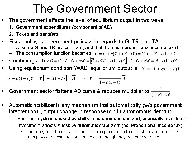
The Government Sector • The government affects the level of equilibrium output in two ways: 1. Government expenditures (component of AD) 2. Taxes and transfers • Fiscal policy is government policy with regards to G, TR, and TA – Assume G and TR are constant, and that there is a proportional income tax (t) – The consumption function becomes: • Combining with • Using equilibrium condition Y=AD, equilibrium output is: • Government sector flattens AD curve & reduces multiplier to • Automatic stabilizer is any mechanism that automatically (w/o government intervention) ↓ output change in response to ↑ in autonomous demand – Business cycle is caused by shifts in autonomous demand, especially investment – Investment affects Y less w/ automatic stabilizers (ex. Proportional income tax) • Unemployment benefits are another example of an automatic stabilizer enables unemployed to continue consuming even though they do not have a job
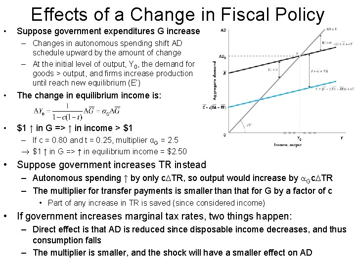
Effects of a Change in Fiscal Policy • Suppose government expenditures G increase – Changes in autonomous spending shift AD schedule upward by the amount of change – At the initial level of output, Y 0, the demand for goods > output, and firms increase production until reach new equilibrium (E’) • The change in equilibrium income is: • $1 ↑ in G => ↑ in income > $1 – If c = 0. 80 and t = 0. 25, multiplier αG = 2. 5 $1 ↑ in G => ↑ in equilibrium income = $2. 50 • Suppose government increases TR instead – Autonomous spending ↑ by only c TR, so output would increase by Gc TR – The multiplier for transfer payments is smaller than that for G by a factor of c • Part of any increase in TR is saved (since considered income) • If government increases marginal tax rates, two things happen: – Direct effect is that AD is reduced since disposable income decreases, and thus consumption falls – The multiplier is smaller, and the shock will have a smaller effect on AD
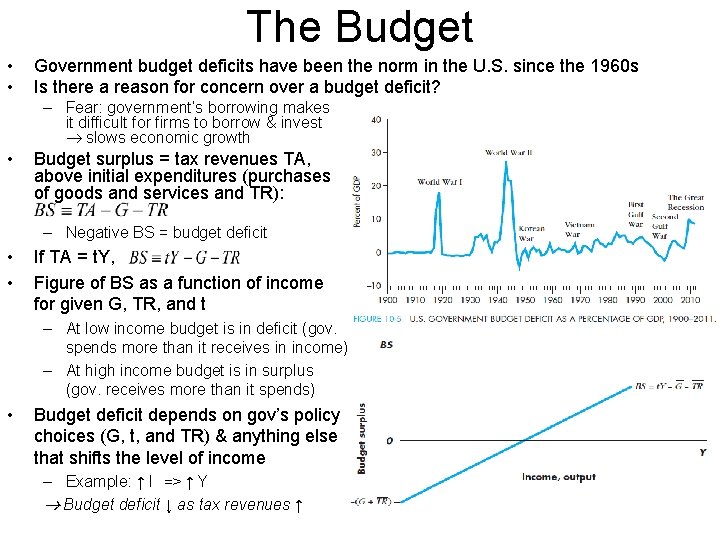
The Budget • • Government budget deficits have been the norm in the U. S. since the 1960 s Is there a reason for concern over a budget deficit? – Fear: government’s borrowing makes it difficult for firms to borrow & invest slows economic growth • Budget surplus = tax revenues TA, above initial expenditures (purchases of goods and services and TR): – Negative BS = budget deficit • • If TA = t. Y, Figure of BS as a function of income for given G, TR, and t – At low income budget is in deficit (gov. spends more than it receives in income) – At high income budget is in surplus (gov. receives more than it spends) • Budget deficit depends on gov’s policy choices (G, t, and TR) & anything else that shifts the level of income – Example: ↑ I => ↑ Y Budget deficit ↓ as tax revenues ↑
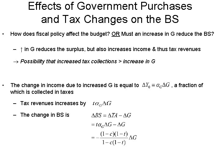
Effects of Government Purchases and Tax Changes on the BS • How does fiscal policy affect the budget? OR Must an increase in G reduce the BS? – ↑ in G reduces the surplus, but also increases income & thus tax revenues Possibility that increased tax collections > increase in G • The change in income due to increased G is equal to which is collected in taxes – Tax revenues increases by – The change in BS is , a fraction of
- Slides: 9