INCA Nowcasting system RTC Training Israel November 2017

INCA Nowcasting system RTC Training, Israel November 2017

The lecture topics: • System background • Infrastructure & I/O • Products

System Background

System background • INCA – Integrated Nowcasting through Comprehensive Analysis. • Developed by ZAMG: http: //www. zamg. ac. at/fix/INCA_system. pdf • IMS joined INCA-CE project in 2011. • Operational mode since 2013

System background System input Automatic Weather Station Observation measurements Numerical Weather Prediction Model forecast Weather RADAR Meteorological Satellite INCA System output Nowcast – short range forecast

System background The added value of the system: • High resolution and Bias correction. • Nowcasting. • Improvement of the short range forecast (first 6 hours) and in farther forecasting range.

System background A look “Inside” INCA Temperature & Humidity module Input NWP processing module Forecasted field Wind module Stations/RADAR/Satellite Forecasted field n’th module

System background NWP processing module Reads the NWP model fields and Interpolates them to INCA levels and grid: • Spatial resolution: 1 km/100 m (Lambert Conic Conformal projection). • Vertical resolution: 200 m to all fields, except for wind 125 m. • Forecast time resolution: 10 minutes/Hourly basis. Processing includes 2 D and 3 D interpolation. The fields on INCA grid are being used by the system’s module to create the Nowcast.
: considers the closest 2 x 2 neighborhood of known")
System background Bilinear interpolation (wikipedia): considers the closest 2 x 2 neighborhood of known pixel values surrounding the unknown pixel's computed location. It then takes a weighted average of these 4 pixels to arrive at its final, interpolated value. The weight on each of the 4 pixel values is based on the computed pixel's distance (in 2 D space) from each of the known points. http: //en. wikipedia. org/wiki/Bilinear_interpolation 9
: is the extension of linear interpolation, which operates in")
System background Trilinear interpolation (wikipedia): is the extension of linear interpolation, which operates in spaces with dimension D = 1, and bilinear interpolation, which operates with dimension D = 2, to dimension D = 3. http: //en. wikipedia. org/wiki/Trilinear_interpolation First we interpolate along z (imagine we are pushing the front face of the cube to the back), giving: Then we interpolate these values (along y, as we were pushing the top edge to the bottom), giving: Finally we interpolate these values along x (walking through a line): 10

System background

System background

System background IMS

System background Module name Output field Timing Temperature & Humidity Analysis & Forecast at 2 m: Temperature, Relative Humidity, Heat Stress, Dew point Temperature, Snowfall line + freezing level Hourly Surface Temperature Analysis & Forecast at the surface (composite with satellite data) Hourly Wind Analysis & Forecast at 10 m Hourly Wind chill Analysis & Forecast Hourly Precipitation Analysis & Forecast: Precipitation, snow, precipitation type. 10 minutes At IMS, precipitation analysis are produced separately in operational mode, based on systems algorithm. Instability indexs CAPE, CIN, LCL … Analysis & Forecast (option forecast developed by IMS) Hourly Cloudiness Analysis & Forecast of cloud cover 15 minutes Icing potential Analysis & Forecast Hourly

System background The different modules take into account: • physical effect of the topography. • change of temperature gradient at the boundary layer.

System background The different modules take into account continue: • the heating/cooling of the surface during the day/night. • the differences between the NWP to the Observations. • Mass conservation during the wind flow. • The effect of AWS one on the other. • The effect of orography on precipitation… etc.

System background The Analysis & Forecast maps are in 1 km/100 m resolution. The forecast range is defined by the user First 6 -12 hours are combination of system and NWP The rest of the forecast range – donation of the NWP downscaled to INCA’s grid and topography

System background Averaged on 88 AWS for the month of june INCA Analysis NWP INCA forecast

System background

Infrastructure & I/O
. •")
Infrastructure & I/O • Linux based system. • Serial computing (in export version). • Bash shell scripts wrapping c and Fortran code. • At IMS graphics output is with Python and GRADS.

Infrastructure & I/O

Infrastructure & I/O

Infrastructure & I/O Numerical Prediction Model Input: • GRIB 1 format • Hourly basis • At IMS: ECMWF/COSMO • 2 D & 3 D fields: temperature, precipitation, etc. • Convention: ECMWF+000. grb…. ECMWF+012. grb

Infrastructure & I/O Automatic Weather Station Input: • Hourly/10 minutes • At IMS, database mining using ad-hoc pearl script. • Text file including gathered measurements from stations observation. • Meta data file regarding stations: geographic location, altitude, etc.

Infrastructure & I/O RADAR data input: • Raw data • Post processed: clutter filtering, CAPPI 1 km product. • 5 minutes basis.
 files")
Infrastructure & I/O System output: • ASCII files • BIL (Binary Interpolated ) files – simple binary file without header. • Images • Post-procced data: Meteograms, PDF

Infrastructure & I/O INCA wind module example

Infrastructure & I/O

Infrastructure & I/O The stages of calculating wind at 10 m: 1. Reading INCA topography and land use (Surface type). 2. Calculating f 10 factor. 3. Reading stations metadata. 4. Getting precipitation data for effect on wind calculation – optional. 5. Defining system levels. 6. Calculating shaved elements. 7. Reading data stations observations. 8. Reading data from Radio-Sonda - optional. 9. Reading the NWP wind fields in INCA levels and grid.

Infrastructure & I/O The stages of calculating wind at 10 m - continue: 10. Finding wind differences between the NWP and stations. 11. Finding wind differences between the NWP and Radio-Sonda - optional. 12. Creating NWP/OBS interpolated differences map. 13. Creating Precipitation wind effect interpolated map – optional. 14. Adding relaxation procedure – mass conservation 15. Creating wind at 10 m adding “lake” effect. 16. Writing modules output fields as ASCII and BIL files.

Infrastructure & I/O f 10 factor calculation – depends on differences between the INCA and the NWP topography

Infrastructure & I/O IDW Interpolation of the NWP and station wind differences Example is taken from the temperature IDW. Same is done for the wind. Constants for wind are n=4 and c=20. . (INCA_system. pdf)

Infrastructure & I/O Shave elements method is used for Mass conservation calculation . (INCA_system. pdf) (2011_Haiden_et_al. pdf)

Infrastructure & I/O from DWD slide show about z coordinate system and shaved elements
מתוך")
Infrastructure & I/O Mass Conservation . (INCA_system. pdf )מתוך

Infrastructure & I/O Adding the “lake” effect

Infrastructure & I/O

Infrastructure & I/O Forecast is created by using weights between INCA Analysis and NWP

Products

products INCA system customers: Israel Meteorological Service: • Forecasting department/operation center - INCA maps, Forecast to Airfields, NWP/OBS auto-check. • Research & Development department - evapotranspiration , radiation calculations. • Climate department Chemical Hazard spill application Israel Hydrology Service/Water Authority INCA precipitation analysis coupled with Hydrological model. Israel fire fighters/Police/Road Safety Agency TV channels The public

products Snow case 19 -20/02/2015

products

products

products Grus in Snowing “Hola” valley http: //www. nrg. co. il/online/1/ART 2/678/158. html

products Nowcast for Airfields

products

products Severe storm case 7/5/2014

products

products From INCA_system. pdf

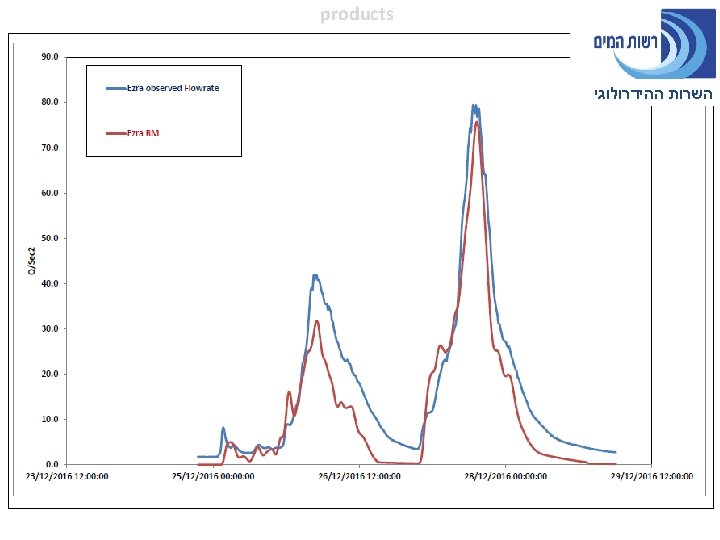
products INCA precipitation coupled to Hydrological model

products Ayalon Basin: division to sub-basin and flow junction in HEC-HMS hydrological model השרות ההידרולוגי

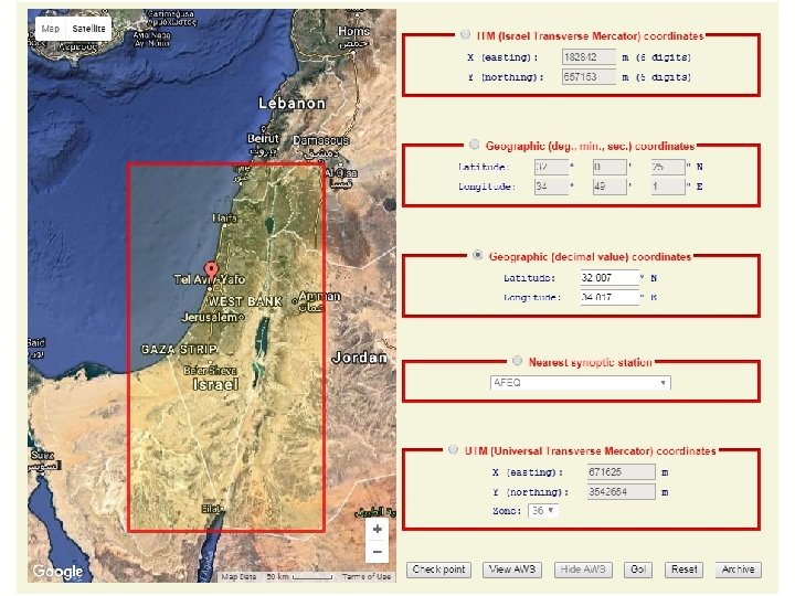
products Chemical spill Hazard application

products

products Summer case

products

Thank you for listening!
- Slides: 59