In the once upon a time days of







- Slides: 86

In the once upon a time days of the First Age of Magic, the prudent sorcerer regarded his own true name as his most valued possession but also the greatest threat to his continued good health, for--the stories go-once an enemy, even a weak unskilled enemy, learned the sorcerer's true name, then routine and widely known spells could destroy or enslave even the most powerful. As times passed, and we graduated to the Age of Reason and thence to the first and second industrial revolutions, such notions were discredited. Now it seems that the Wheel has turned full circle (even if there never really was a First Age) and we are back to worrying about true names again: The first hint Mr. Slippery had that his own True Name might be known-and, for that matter, known to the Great Enemy--came with the appearance of two black Lincolns humming up the long dirt driveway. . . Roger Pollack was in his garden weeding, had been there nearly the whole morning. . Four heavy-set men and a hard-looking female piled out, started purposefully across his well-tended cabbage patch. … This had been, of course, Roger Pollack's great fear. They had discovered Mr. Slippery's True Name and it was Roger Andrew Pollack TIN/SSAN 0959 -34 -2861. 1

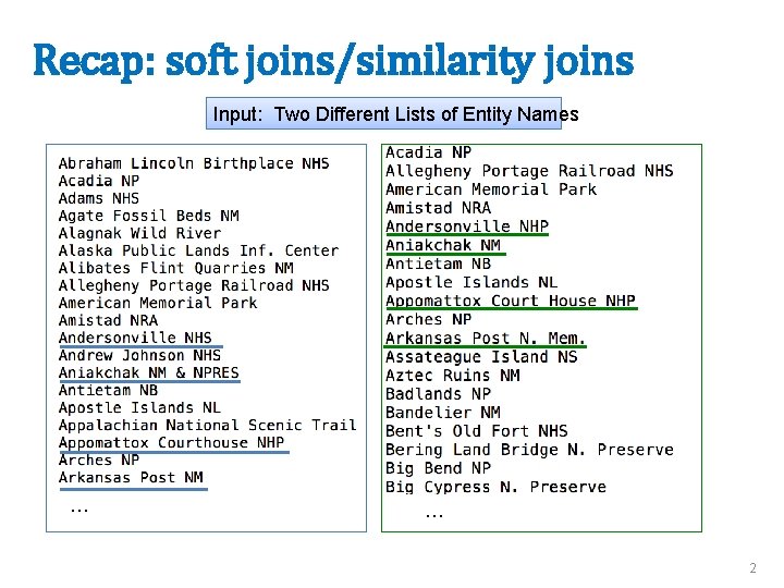
Recap: soft joins/similarity joins Input: Two Different Lists of Entity Names … … 2

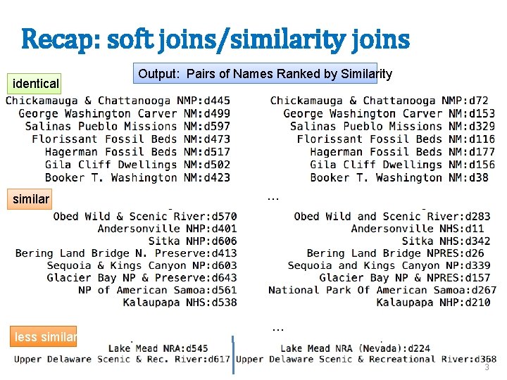
Recap: soft joins/similarity joins identical similar less similar Output: Pairs of Names Ranked by Similarity … … 3

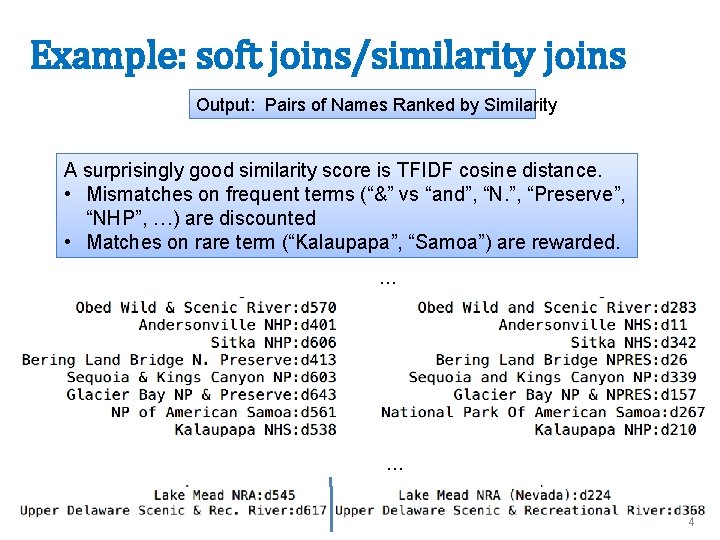
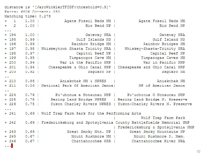
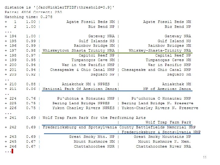
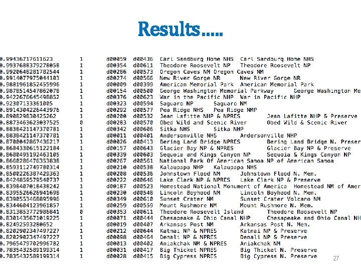
Example: soft joins/similarity joins Output: Pairs of Names Ranked by Similarity A surprisingly good similarity score is TFIDF cosine distance. • Mismatches on frequent terms (“&” vs “and”, “N. ”, “Preserve”, “NHP”, …) are discounted • Matches on rare term (“Kalaupapa”, “Samoa”) are rewarded. … … 4

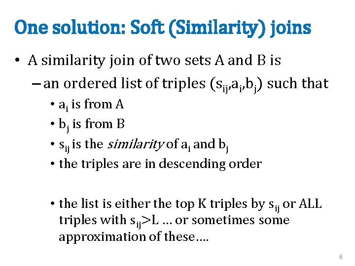
One solution: Soft (Similarity) joins • A similarity join of two sets A and B is – an ordered list of triples (sij, ai, bj) such that • ai is from A • bj is from B • sij is the similarity of ai and bj • the triples are in descending order • the list is either the top K triples by sij or ALL triples with sij>L … or sometimes some approximation of these…. 6

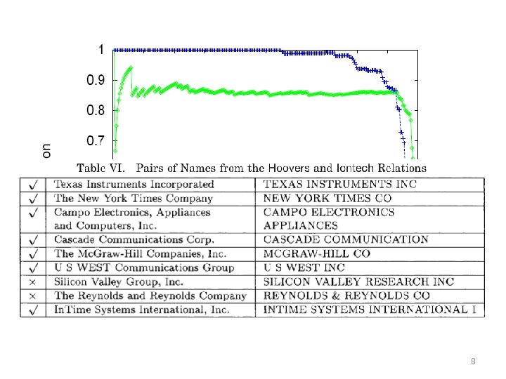
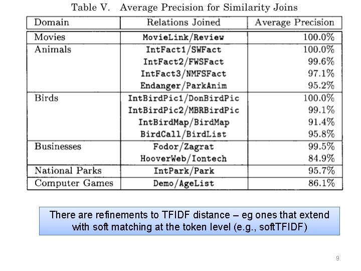
How well does TFIDF work? 7

8

There are refinements to TFIDF distance – eg ones that extend with soft matching at the token level (e. g. , soft. TFIDF) 9

Semantic Joining with Multiscale Statistics William Cohen Katie Rivard, Dana Attias-Moshevitz CMU 10

Semantic Joining with Multiscale Statistics William Cohen Katie Rivard, Dana Attias-Moshevitz CMU 11

SOFT JOINS WITH TFIDF: HOW? 12

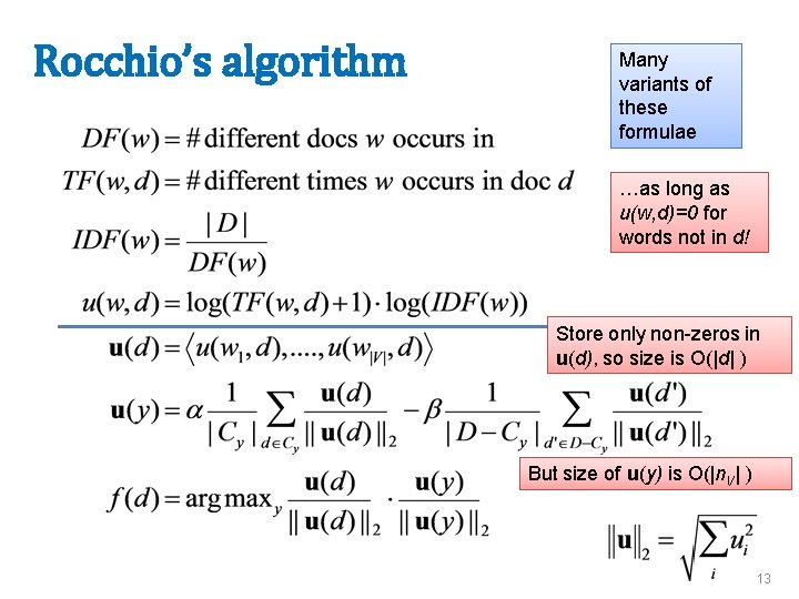
Rocchio’s algorithm Many variants of these formulae …as long as u(w, d)=0 for words not in d! Store only non-zeros in u(d), so size is O(|d| ) But size of u(y) is O(|n. V| ) 13

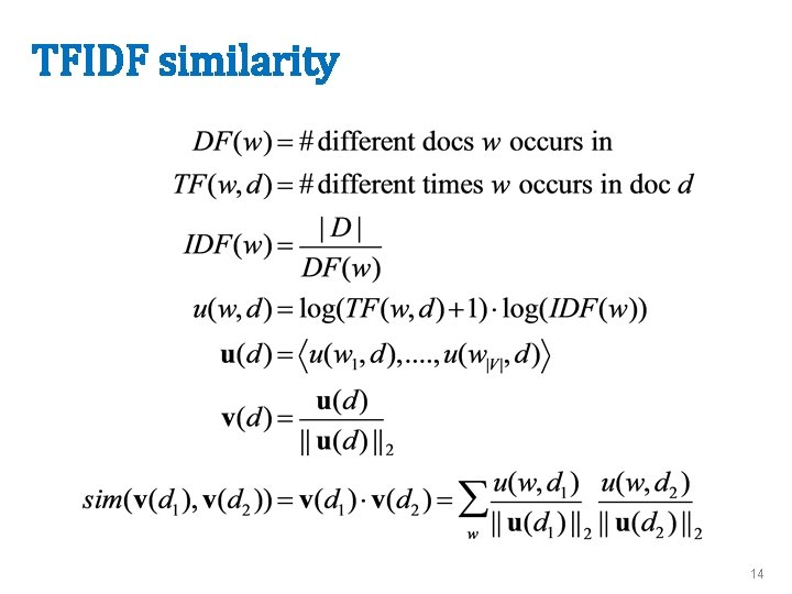
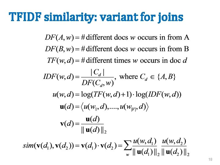
TFIDF similarity 14

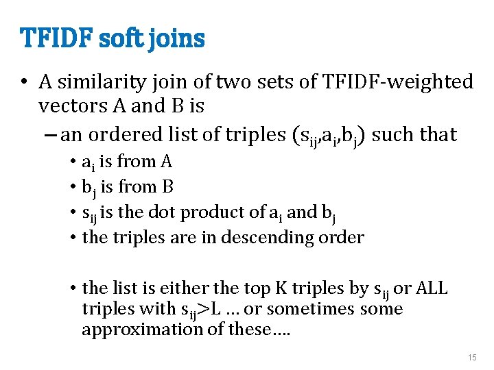
TFIDF soft joins • A similarity join of two sets of TFIDF-weighted vectors A and B is – an ordered list of triples (sij, ai, bj) such that • ai is from A • bj is from B • sij is the dot product of ai and bj • the triples are in descending order • the list is either the top K triples by sij or ALL triples with sij>L … or sometimes some approximation of these…. 15

PARALLEL SOFT JOINS 16

SIGMOD 2010 17

TFIDF similarity: variant for joins 18

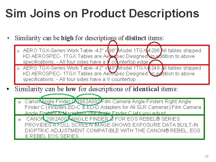
Sim Joins on Product Descriptions • Similarity can be high for descriptions of distinct items: AERO TGX-Series Work Table -42'' x 96'' Model 1 TGX-4296 All tables shipped KD AEROSPEC- 1 TGX Tables are Aerospec Designed. In addition to above specifications; - All four sides have a V countertop edge. . . o AERO TGX-Series Work Table -42'' x 48'' Model 1 TGX-4248 All tables shipped KD AEROSPEC- 1 TGX Tables are Aerospec Designed. In addition to above specifications; - All four sides have a V countertop. . o • Similarity can be low for descriptions of identical items: Canon Angle Finder C 2882 A 002 Film Camera Angle Finders Right Angle Finder C (Includes ED-C & ED-D Adapters for All SLR Cameras) Film Camera Angle Finders & Magnifiers The Angle Finder C lets you adjust . . . o CANON 2882 A 002 ANGLE FINDER C FOR EOS REBEL® SERIES PROVIDES A FULL SCREEN IMAGE SHOWS EXPOSURE DATA BUILT-IN DIOPTRIC ADJUSTMENT COMPATIBLE WITH THE CANON® REBEL, EOS & REBEL EOS SERIES. o 19

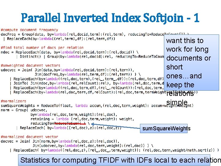
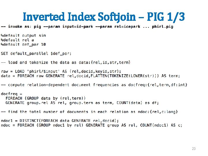
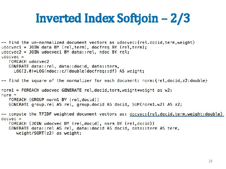
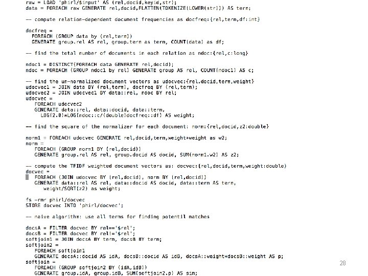
Parallel Inverted Index Softjoin - 1 want this to work for long documents or short ones…and keep the relations simple sum. Square. Weights 20 Statistics for computing TFIDF with IDFs local to each relation

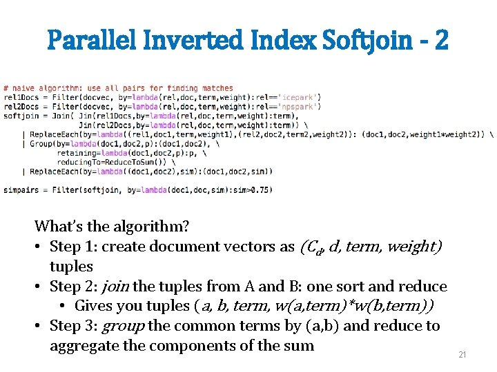
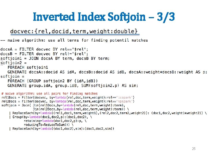
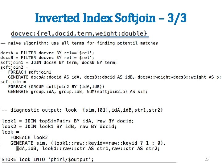
Parallel Inverted Index Softjoin - 2 What’s the algorithm? • Step 1: create document vectors as (Cd, d, term, weight) tuples • Step 2: join the tuples from A and B: one sort and reduce • Gives you tuples (a, b, term, w(a, term)*w(b, term)) • Step 3: group the common terms by (a, b) and reduce to aggregate the components of the sum 21

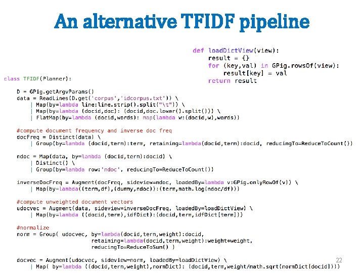
An alternative TFIDF pipeline 22

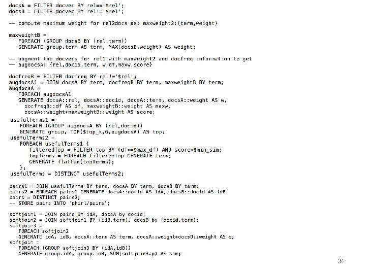
Inverted Index Softjoin – PIG 1/3 23

Inverted Index Softjoin – 2/3 24

Inverted Index Softjoin – 3/3 25

Inverted Index Softjoin – 3/3 26

Results…. . 27

28

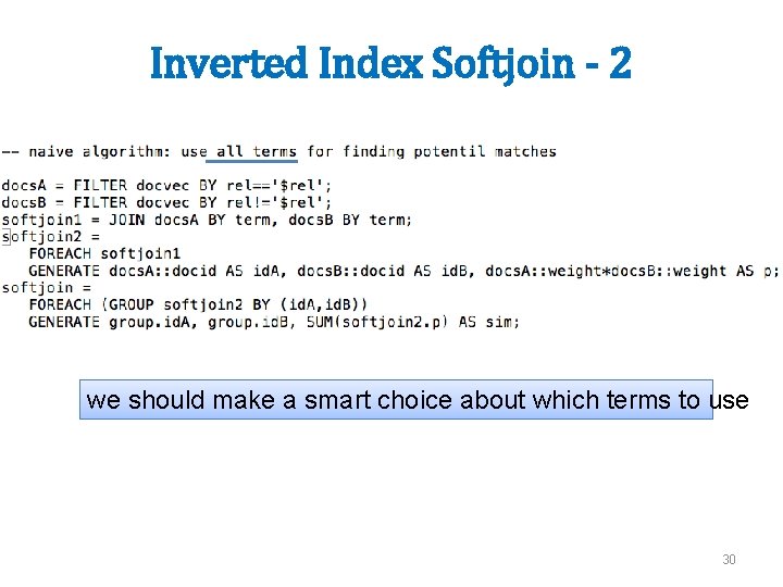
Making the algorithm smarter…. 29

Inverted Index Softjoin - 2 we should make a smart choice about which terms to use 30

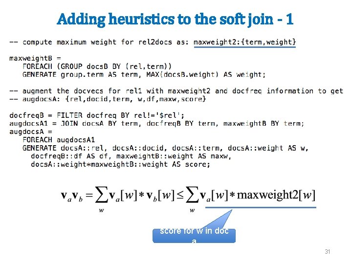
Adding heuristics to the soft join - 1 score for w in doc a 31

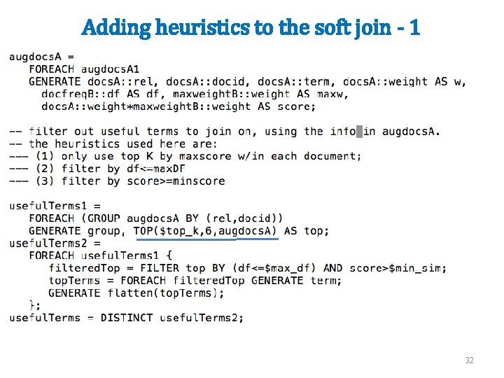
Adding heuristics to the soft join - 1 32

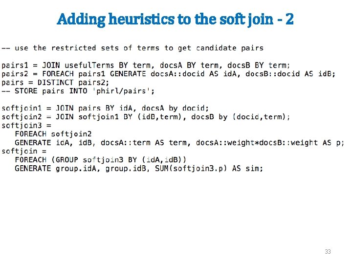
Adding heuristics to the soft join - 2 33

34

Page. Rank at Scale 35

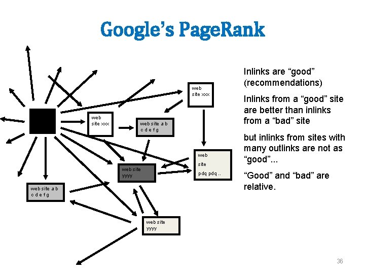
Google’s Page. Rank web site xxx web site a b c d e f g web site yyyy pdq. . web site a b c d e f g Inlinks are “good” (recommendations) Inlinks from a “good” site are better than inlinks from a “bad” site but inlinks from sites with many outlinks are not as “good”. . . “Good” and “bad” are relative. web site yyyy 36

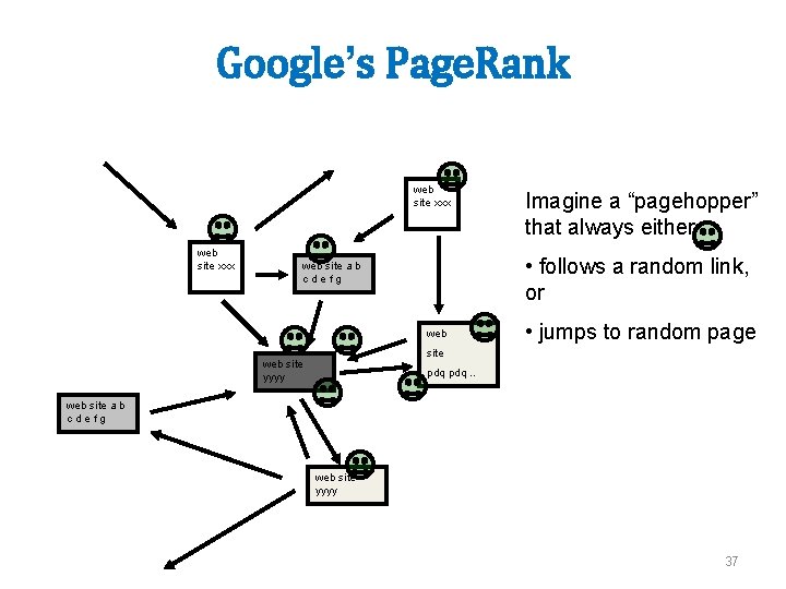
Google’s Page. Rank web site xxx Imagine a “pagehopper” that always either • follows a random link, or web site a b c d e f g web • jumps to random page site web site yyyy pdq. . web site a b c d e f g web site yyyy 37

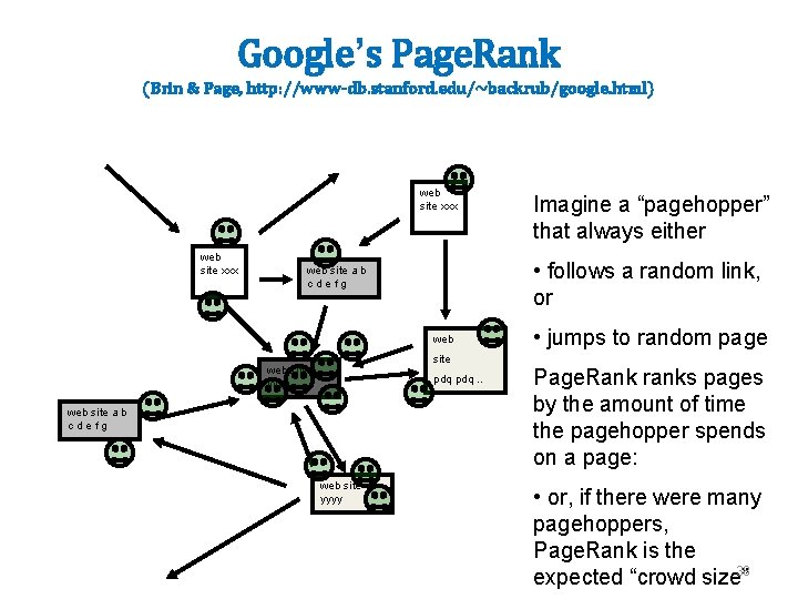
Google’s Page. Rank (Brin & Page, http: //www-db. stanford. edu/~backrub/google. html) web site xxx • follows a random link, or web site a b c d e f g web site yyyy pdq. . web site a b c d e f g web site yyyy Imagine a “pagehopper” that always either • jumps to random page Page. Rank ranks pages by the amount of time the pagehopper spends on a page: • or, if there were many pagehoppers, Page. Rank is the 38 expected “crowd size”

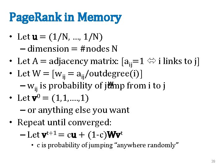
Page. Rank in Memory • Let u = (1/N, …, 1/N) – dimension = #nodes N • Let A = adjacency matrix: [aij=1 i links to j] • Let W = [wij = aij/outdegree(i)] W – wij is probability of jump from i to j • Let v 0 = (1, 1, …. , 1) – or anything else you want • Repeat until converged: – Let vt+1 = cu + (1 -c)Wvt • c is probability of jumping “anywhere randomly” 39

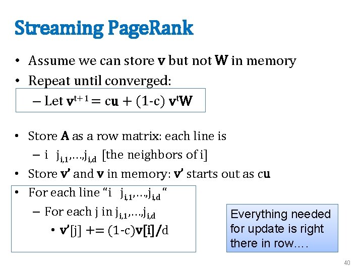
Streaming Page. Rank • Assume we can store v but not W in memory • Repeat until converged: – Let vt+1 = cu + (1 -c) vt. W • Store A as a row matrix: each line is – i ji, 1, …, ji, d [the neighbors of i] • Store v’ and v in memory: v’ starts out as cu • For each line “i ji, 1, …, ji, d “ – For each j in ji, 1, …, ji, d Everything needed for update is right • v’[j] += (1 -c)v[i]/d there in row…. 40

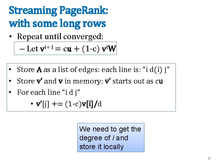
Streaming Page. Rank: with some long rows • Repeat until converged: – Let vt+1 = cu + (1 -c) vt. W • Store A as a list of edges: each line is: “i d(i) j” • Store v’ and v in memory: v’ starts out as cu • For each line “i d j“ • v’[j] += (1 -c)v[i]/d We need to get the degree of i and store it locally 41

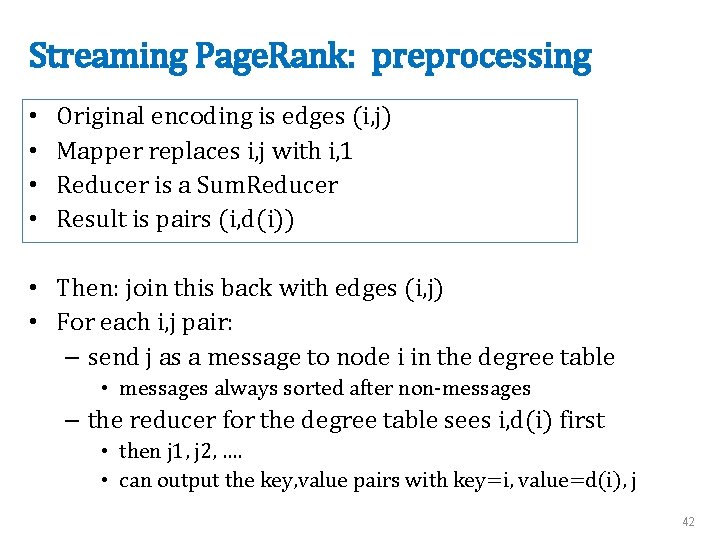
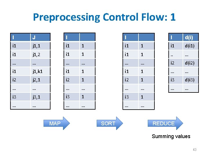
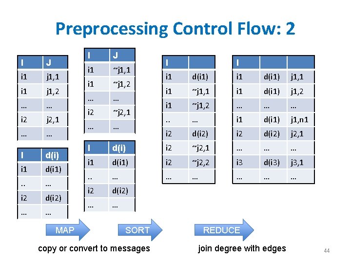
Streaming Page. Rank: preprocessing • • Original encoding is edges (i, j) Mapper replaces i, j with i, 1 Reducer is a Sum. Reducer Result is pairs (i, d(i)) • Then: join this back with edges (i, j) • For each i, j pair: – send j as a message to node i in the degree table • messages always sorted after non-messages – the reducer for the degree table sees i, d(i) first • then j 1, j 2, …. • can output the key, value pairs with key=i, value=d(i), j 42

Preprocessing Control Flow: 1 I J I i 1 j 1, 1 i 1 i 1 j 1, 2 i 1 1 … … … i 1 j 1, k 1 i 2 I d(i) 1 i 1 d(i 1) i 1 1 . . … … i 2 d(i 2) i 1 1 … … j 2, 1 i 2 1 i 3 d)i 3) … … … … i 3 j 3, 1 i 3 1 … … … MAP I SORT REDUCE Summing values 43

Preprocessing Control Flow: 2 I J i 1 j 1, 1 i 1 j 1, 2 … … i 2 j 2, 1 … … I d(i) i 1 d(i 1) . . … i 2 d(i 2) … … MAP I J i 1 ~j 1, 1 i 1 ~j 1, 2 … … i 2 ~j 2, 1 … … I I I i 1 d(i 1) j 1, 1 i 1 ~j 1, 1 i 1 d(i 1) j 1, 2 i 1 ~j 1, 2 … … … . . … i 1 d(i 1) j 1, n 1 i 2 d(i 2) j 2, 1 d(i) i 2 ~j 2, 1 … … … i 1 d(i 1) i 2 ~j 2, 2 i 3 d(i 3) j 3, 1 . . … … … i 2 d(i 2) … … SORT copy or convert to messages REDUCE join degree with edges 44

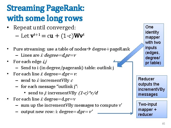
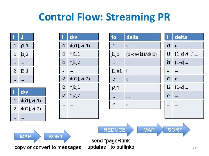
Streaming Page. Rank: with some long rows • Repeat until converged: – Let vt+1 = cu + (1 -c)Wvt • Pure streaming: use a table of nodes degree+page. Rank – Lines are i: degree=d, pr=v • For each edge i, j – Send to i (in degree/pagerank) table: outlink j • For each line i: degree=d, pr=v: – send to i: increment. VBy c – for each message “outlink j”: • send to j: increment. VBy (1 -c)*v/d • For each line i: degree=d, pr=v – sum up the increment. VBy messages to compute v’ – output new row: i: degree=d, pr=v’ One identity mapper with two inputs (edges, degree/ pr table) Reducer outputs the increment. VBy messages Two-input mapper + reducer 45

Control Flow: Streaming PR I J I d/v to delta I delta i 1 j 1, 1 i 1 d(i 1), v(i 1) i 1 c i 1 j 1, 2 i 1 ~j 1, 1 (1 -c)v(i 1)/d(i 1) i 1 (1 -c)v(…)…. … … i 1 ~j 1, 2 … … i 1 (1 -c)… i 2 j 2, 1 . . j 1, n 1 i . . … … i 2 d(i 2), v(i 2) i 2 c i 2 ~j 2, 1 … i 2 (1 -c)… i 2 ~j 2, 2 … … i 2 …. … … i 3 c … … I d/v i 1 d(i 1), v(i 1) i 2 d(i 2), v(i 2) … … REDUCE MAP SORT copy or convert to messages send “page. Rank updates ” to outlinks MAP SORT 46

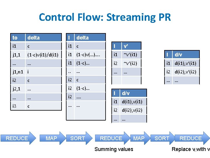
Control Flow: Streaming PR to delta I delta i 1 c I v’ j 1, 1 (1 -c)v(i 1)/d(i 1) i 1 (1 -c)v(…)…. i 1 ~v’(i 1) I … … i 1 (1 -c)… i 2 ~v’(i 2) i 1 d(i 1), v’(i 1) j 1, n 1 i . . … … i 2 d(i 2), v’(i 2) i 2 c j 2, 1 … i 2 (1 -c)… … … i 2 …. i 3 c … … … d/v … … I d/v i 1 d(i 1), v(i 1) i 2 d(i 2), v(i 2) … … REDUCE MAP SORT REDUCE MAP Summing values SORT REDUCE Replace v with v’ 47

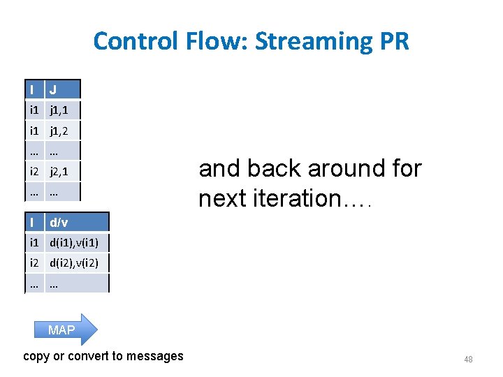
Control Flow: Streaming PR I J i 1 j 1, 1 i 1 j 1, 2 … … i 2 j 2, 1 … … I and back around for next iteration…. d/v i 1 d(i 1), v(i 1) i 2 d(i 2), v(i 2) … … MAP copy or convert to messages 48

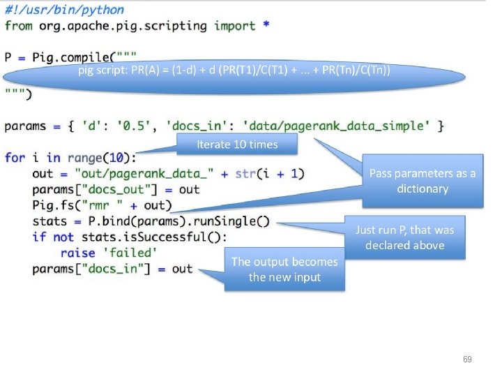
Page. Rank in Pig 49

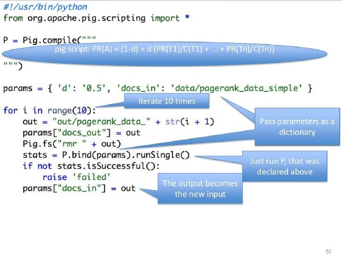
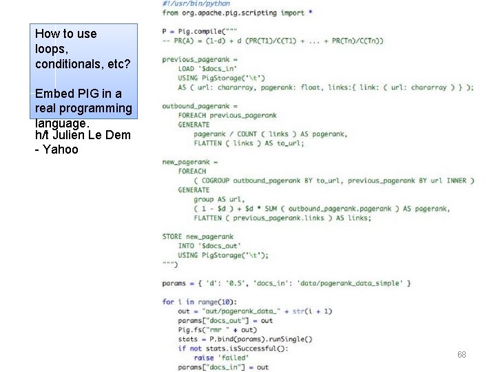
How to use loops, conditionals, etc? Embed PIG in a real programming language. Julien Le Dem - Yahoo 50

51

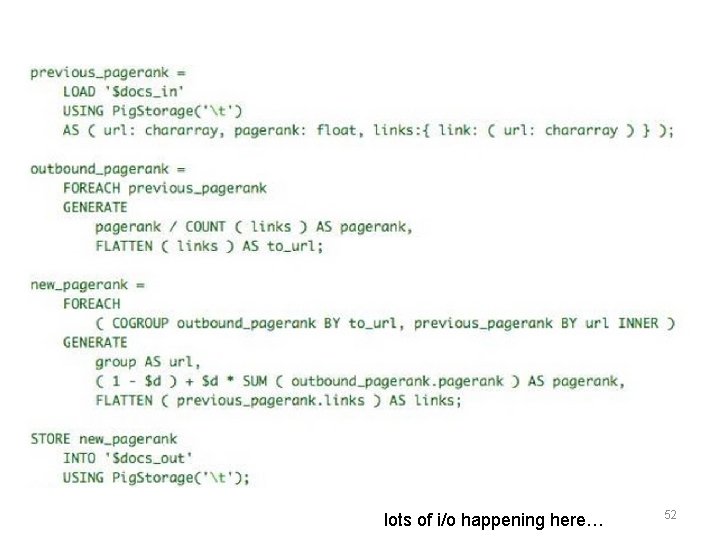
lots of i/o happening here… 52

An example from Ron Bekkerman 53

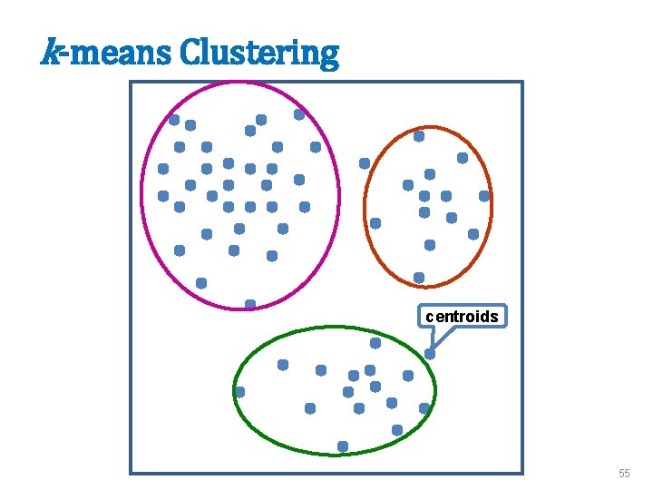
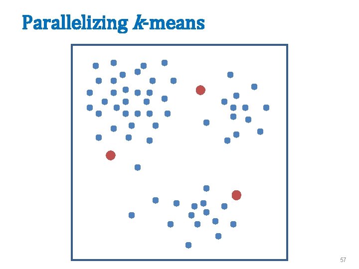
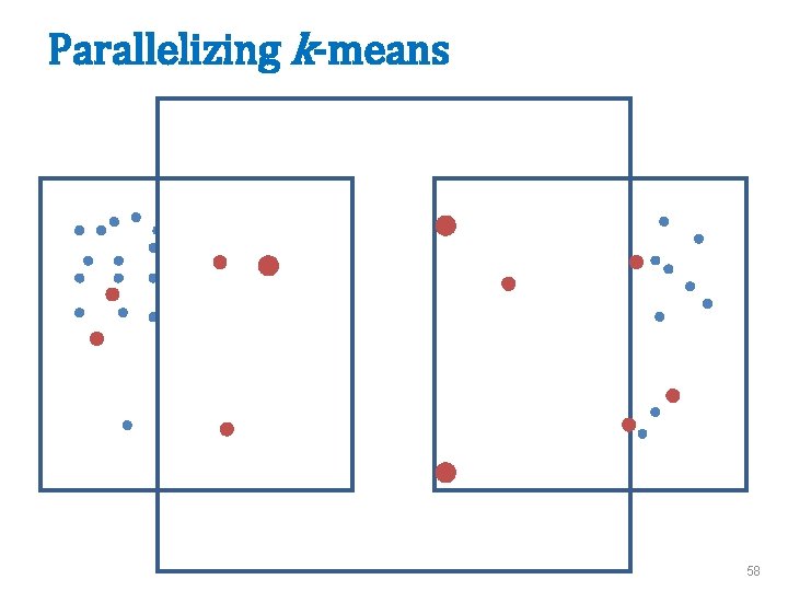
Example: k-means clustering • An EM-like algorithm: • Initialize k cluster centroids • E-step: associate each data instance with the closest centroid – Find expected values of cluster assignments given the data and centroids • M-step: recalculate centroids as an average of the associated data instances – Find new centroids that maximize that expectation 54

k-means Clustering centroids 55

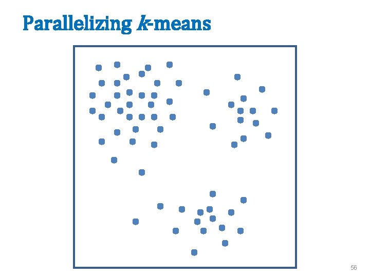
Parallelizing k-means 56

Parallelizing k-means 57

Parallelizing k-means 58

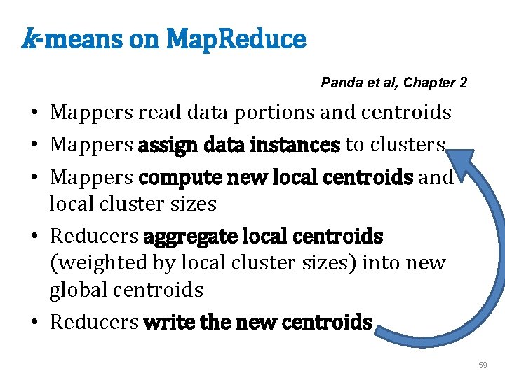
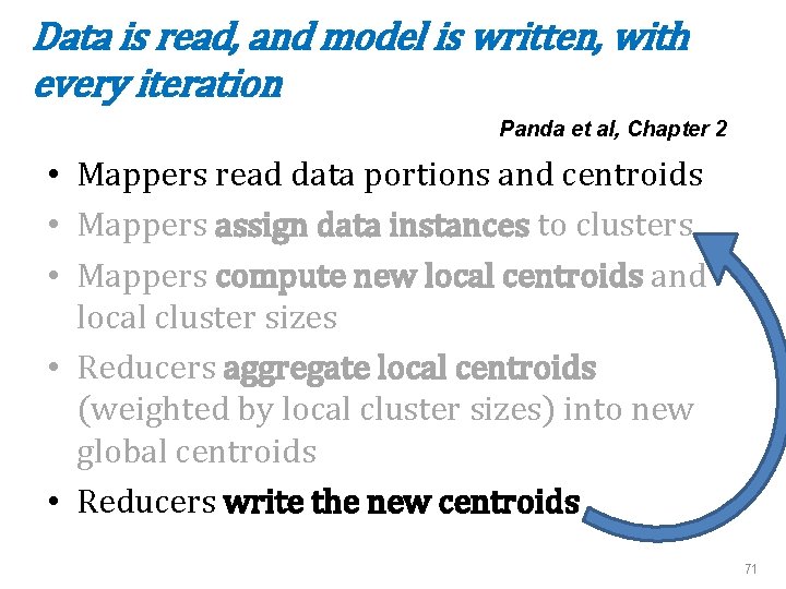
k-means on Map. Reduce Panda et al, Chapter 2 • Mappers read data portions and centroids • Mappers assign data instances to clusters • Mappers compute new local centroids and local cluster sizes • Reducers aggregate local centroids (weighted by local cluster sizes) into new global centroids • Reducers write the new centroids 59

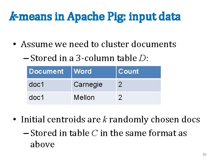
k-means in Apache Pig: input data • Assume we need to cluster documents – Stored in a 3 -column table D: Document Word Count doc 1 Carnegie 2 doc 1 Mellon 2 • Initial centroids are k randomly chosen docs – Stored in table C in the same format as above 60

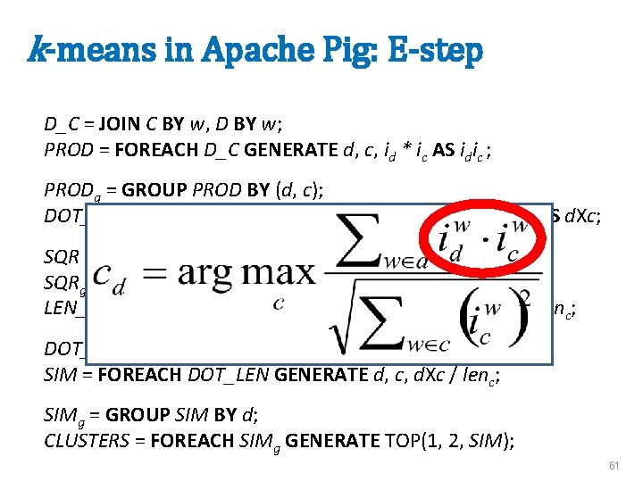
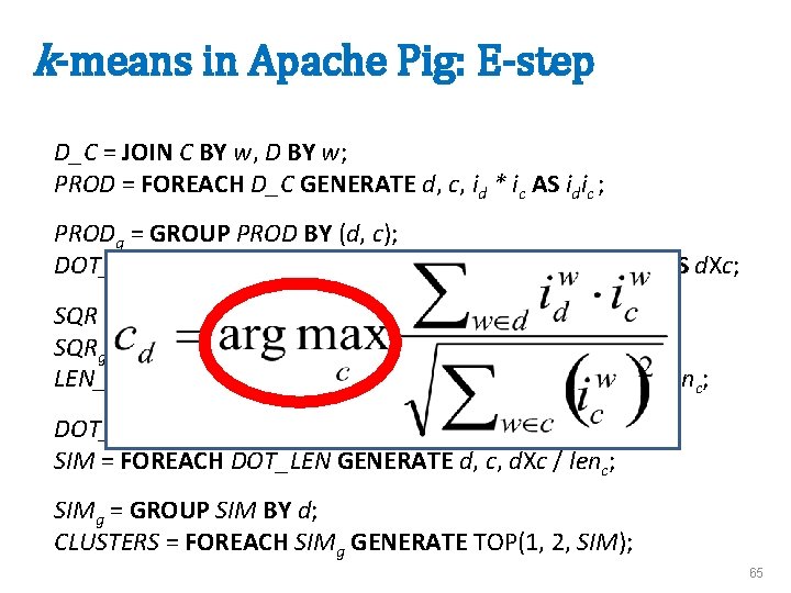
k-means in Apache Pig: E-step D_C = JOIN C BY w, D BY w; PROD = FOREACH D_C GENERATE d, c, id * ic AS idic ; PRODg = GROUP PROD BY (d, c); DOT_PROD = FOREACH PRODg GENERATE d, c, SUM(idic) AS d. Xc; SQR = FOREACH C GENERATE c, ic * ic AS ic 2; SQRg = GROUP SQR BY c; LEN_C = FOREACH SQRg GENERATE c, SQRT(SUM(ic 2)) AS lenc; DOT_LEN = JOIN LEN_C BY c, DOT_PROD BY c; SIM = FOREACH DOT_LEN GENERATE d, c, d. Xc / lenc; SIMg = GROUP SIM BY d; CLUSTERS = FOREACH SIMg GENERATE TOP(1, 2, SIM); 61

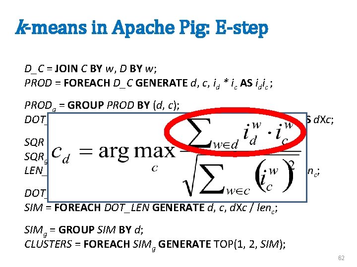
k-means in Apache Pig: E-step D_C = JOIN C BY w, D BY w; PROD = FOREACH D_C GENERATE d, c, id * ic AS idic ; PRODg = GROUP PROD BY (d, c); DOT_PROD = FOREACH PRODg GENERATE d, c, SUM(idic) AS d. Xc; SQR = FOREACH C GENERATE c, ic * ic AS ic 2; SQRg = GROUP SQR BY c; LEN_C = FOREACH SQRg GENERATE c, SQRT(SUM(ic 2)) AS lenc; DOT_LEN = JOIN LEN_C BY c, DOT_PROD BY c; SIM = FOREACH DOT_LEN GENERATE d, c, d. Xc / lenc; SIMg = GROUP SIM BY d; CLUSTERS = FOREACH SIMg GENERATE TOP(1, 2, SIM); 62

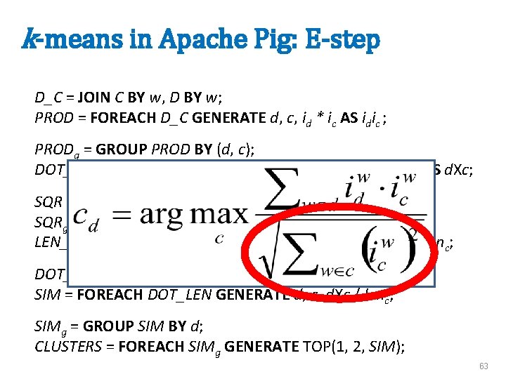
k-means in Apache Pig: E-step D_C = JOIN C BY w, D BY w; PROD = FOREACH D_C GENERATE d, c, id * ic AS idic ; PRODg = GROUP PROD BY (d, c); DOT_PROD = FOREACH PRODg GENERATE d, c, SUM(idic) AS d. Xc; SQR = FOREACH C GENERATE c, ic * ic AS ic 2; SQRg = GROUP SQR BY c; LEN_C = FOREACH SQRg GENERATE c, SQRT(SUM(ic 2)) AS lenc; DOT_LEN = JOIN LEN_C BY c, DOT_PROD BY c; SIM = FOREACH DOT_LEN GENERATE d, c, d. Xc / lenc; SIMg = GROUP SIM BY d; CLUSTERS = FOREACH SIMg GENERATE TOP(1, 2, SIM); 63

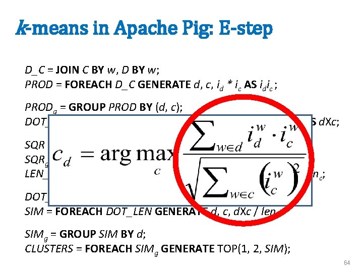
k-means in Apache Pig: E-step D_C = JOIN C BY w, D BY w; PROD = FOREACH D_C GENERATE d, c, id * ic AS idic ; PRODg = GROUP PROD BY (d, c); DOT_PROD = FOREACH PRODg GENERATE d, c, SUM(idic) AS d. Xc; SQR = FOREACH C GENERATE c, ic * ic AS ic 2; SQRg = GROUP SQR BY c; LEN_C = FOREACH SQRg GENERATE c, SQRT(SUM(ic 2)) AS lenc; DOT_LEN = JOIN LEN_C BY c, DOT_PROD BY c; SIM = FOREACH DOT_LEN GENERATE d, c, d. Xc / lenc; SIMg = GROUP SIM BY d; CLUSTERS = FOREACH SIMg GENERATE TOP(1, 2, SIM); 64

k-means in Apache Pig: E-step D_C = JOIN C BY w, D BY w; PROD = FOREACH D_C GENERATE d, c, id * ic AS idic ; PRODg = GROUP PROD BY (d, c); DOT_PROD = FOREACH PRODg GENERATE d, c, SUM(idic) AS d. Xc; SQR = FOREACH C GENERATE c, ic * ic AS ic 2; SQRg = GROUP SQR BY c; LEN_C = FOREACH SQRg GENERATE c, SQRT(SUM(ic 2)) AS lenc; DOT_LEN = JOIN LEN_C BY c, DOT_PROD BY c; SIM = FOREACH DOT_LEN GENERATE d, c, d. Xc / lenc; SIMg = GROUP SIM BY d; CLUSTERS = FOREACH SIMg GENERATE TOP(1, 2, SIM); 65

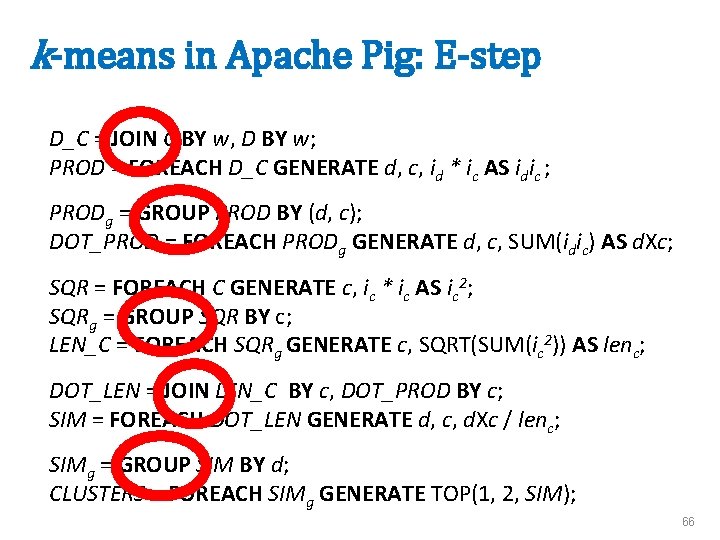
k-means in Apache Pig: E-step D_C = JOIN C BY w, D BY w; PROD = FOREACH D_C GENERATE d, c, id * ic AS idic ; PRODg = GROUP PROD BY (d, c); DOT_PROD = FOREACH PRODg GENERATE d, c, SUM(idic) AS d. Xc; SQR = FOREACH C GENERATE c, ic * ic AS ic 2; SQRg = GROUP SQR BY c; LEN_C = FOREACH SQRg GENERATE c, SQRT(SUM(ic 2)) AS lenc; DOT_LEN = JOIN LEN_C BY c, DOT_PROD BY c; SIM = FOREACH DOT_LEN GENERATE d, c, d. Xc / lenc; SIMg = GROUP SIM BY d; CLUSTERS = FOREACH SIMg GENERATE TOP(1, 2, SIM); 66

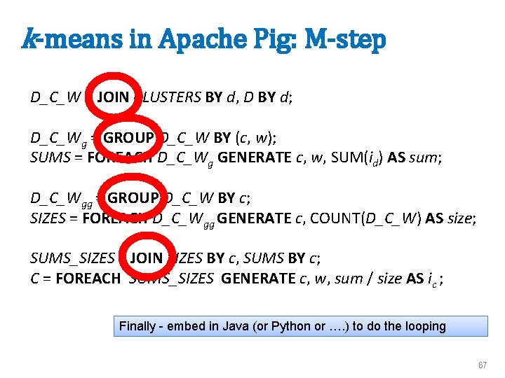
k-means in Apache Pig: M-step D_C_W = JOIN CLUSTERS BY d, D BY d; D_C_Wg = GROUP D_C_W BY (c, w); SUMS = FOREACH D_C_Wg GENERATE c, w, SUM(id) AS sum; D_C_Wgg = GROUP D_C_W BY c; SIZES = FOREACH D_C_Wgg GENERATE c, COUNT(D_C_W) AS size; SUMS_SIZES = JOIN SIZES BY c, SUMS BY c; C = FOREACH SUMS_SIZES GENERATE c, w, sum / size AS ic ; Finally - embed in Java (or Python or …. ) to do the looping 67

How to use loops, conditionals, etc? Embed PIG in a real programming language. h/t Julien Le Dem - Yahoo 68

69

The problem with k-means in Hadoop I/O costs 70

Data is read, and model is written, with every iteration Panda et al, Chapter 2 • Mappers read data portions and centroids • Mappers assign data instances to clusters • Mappers compute new local centroids and local cluster sizes • Reducers aggregate local centroids (weighted by local cluster sizes) into new global centroids • Reducers write the new centroids 71

Spark 72

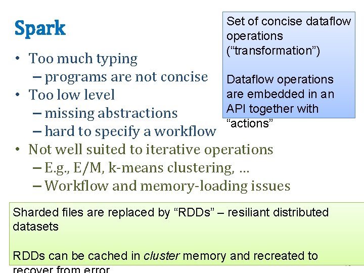
Spark Set of concise dataflow operations (“transformation”) • Too much typing – programs are not concise Dataflow operations are embedded in an • Too low level API together with – missing abstractions “actions” – hard to specify a workflow • Not well suited to iterative operations – E. g. , E/M, k-means clustering, … – Workflow and memory-loading issues Sharded files are replaced by “RDDs” – resiliant distributed datasets RDDs can be cached in cluster memory and recreated to 73

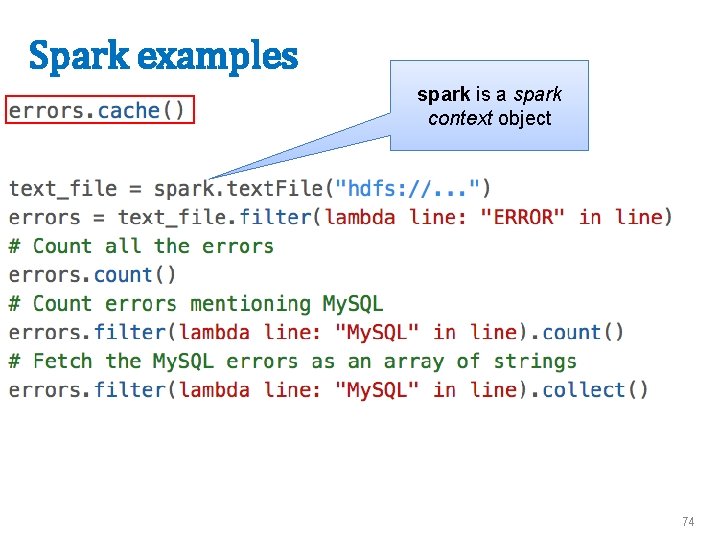
Spark examples spark is a spark context object 74

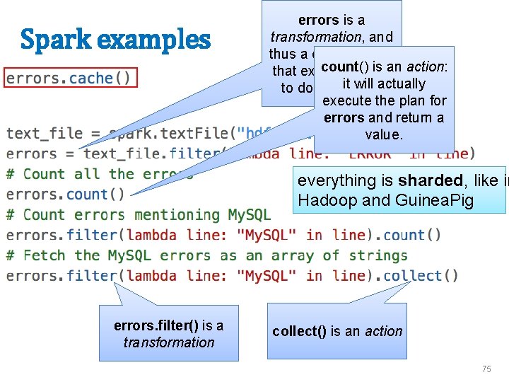
Spark examples errors is a transformation, and thus a data strucure count() is an action: that explains HOW it will actually to do something execute the plan for errors and return a value. everything is sharded, like in Hadoop and Guinea. Pig errors. filter() is a transformation collect() is an action 75

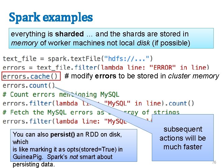
Spark examples everything is sharded … and the shards are stored in memory of worker machines not local disk (if possible) # modify errors to be stored in cluster memory You can also persist() an RDD on disk, which is like marking it as opts(stored=True) in Guinea. Pig. Spark’s not smart about persisting data. subsequent actions will be much faster 76

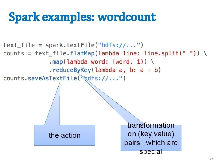
Spark examples: wordcount the action transformation on (key, value) pairs , which are special 77

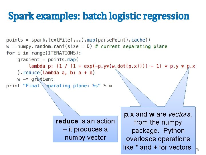
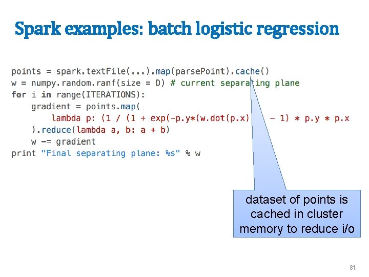
Spark examples: batch logistic regression p. x and w are vectors, from the reduce is an action from the numpy package – it produces a package. Python numby vector overloads operations like * and + for vectors. 78

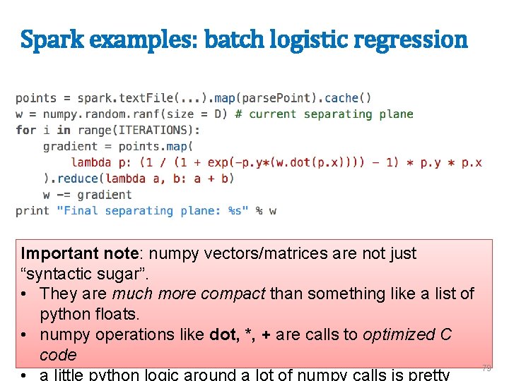
Spark examples: batch logistic regression Important note: numpy vectors/matrices are not just “syntactic sugar”. • They are much more compact than something like a list of python floats. • numpy operations like dot, *, + are calls to optimized C code 79 • a little python logic around a lot of numpy calls is pretty

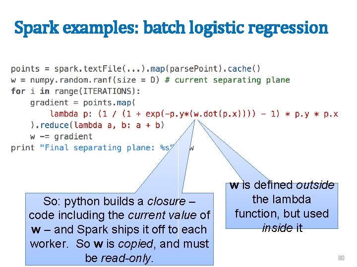
Spark examples: batch logistic regression So: python builds a closure – code including the current value of w – and Spark ships it off to each worker. So w is copied, and must be read-only. w is defined outside the lambda function, but used inside it 80

Spark examples: batch logistic regression dataset of points is cached in cluster memory to reduce i/o 81

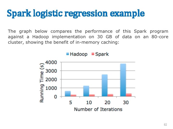
Spark logistic regression example 82

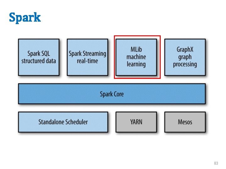
Spark 83

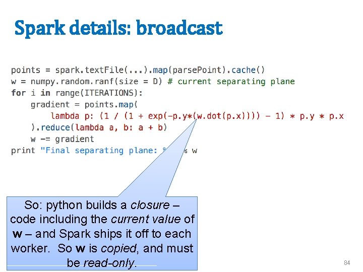
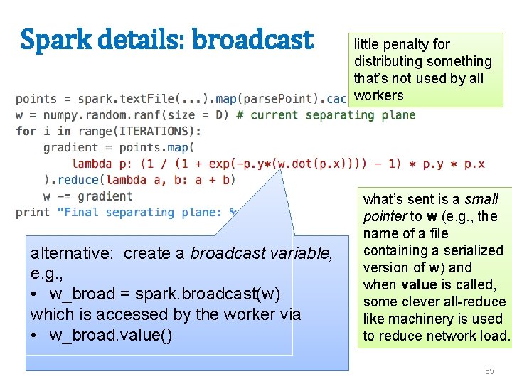
Spark details: broadcast So: python builds a closure – code including the current value of w – and Spark ships it off to each worker. So w is copied, and must be read-only. 84

Spark details: broadcast alternative: create a broadcast variable, e. g. , • w_broad = spark. broadcast(w) which is accessed by the worker via • w_broad. value() little penalty for distributing something that’s not used by all workers what’s sent is a small pointer to w (e. g. , the name of a file containing a serialized version of w) and when value is called, some clever all-reduce like machinery is used to reduce network load. 85

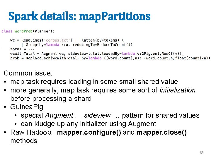
Spark details: map. Partitions Common issue: • map task requires loading in some small shared value • more generally, map task requires some sort of initialization before processing a shard • Guinea. Pig: • special Augment … sideview … pattern for shared values • can kludge up any initializer using Augment • Raw Hadoop: mapper. configure() and mapper. close() methods 86

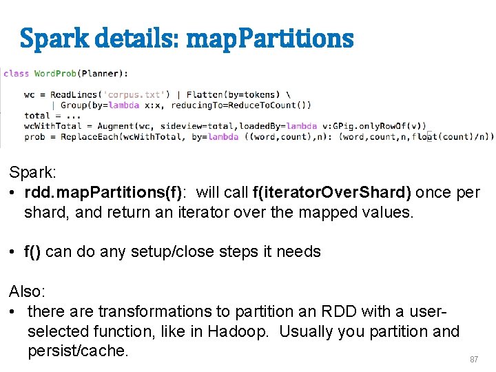
Spark details: map. Partitions Spark: • rdd. map. Partitions(f): will call f(iterator. Over. Shard) once per shard, and return an iterator over the mapped values. • f() can do any setup/close steps it needs Also: • there are transformations to partition an RDD with a userselected function, like in Hadoop. Usually you partition and persist/cache. 87