In Engineering Designing a Pneumatic Pump Introduction System

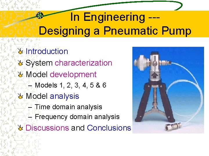
In Engineering --Designing a Pneumatic Pump Introduction System characterization Model development – Models 1, 2, 3, 4, 5 & 6 Model analysis – Time domain analysis – Frequency domain analysis Discussions and Conclusions

Introduction In an aquarium, it is essential that there be a good supply of dissolved oxygen to maintain the health of the fish and other life inside the tank. This if often achieved by pumping air into it. The performance of the pump depends on its design, which in turn involves two phases. – I: Conceptual design in which a suitable scheme s developed ---- this involves identifying the different components and the coupling between components necessary for a solution – Phase II: Specification of components in terms of their size, characteristics and other functional parameters so that the pump performance meets some stated criterion. We concentrate the second phase!!— Predicting the performance of a small pneumatic pump, suitable for domestic aquariums, as a function of the characteristics of its components.

System Characterization

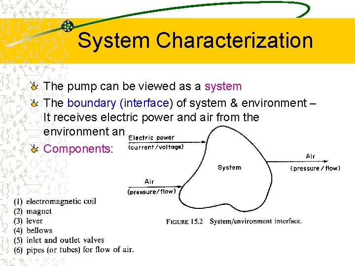
System Characterization The pump can be viewed as a system The boundary (interface) of system & environment – It receives electric power and air from the environment and supplies air to the aquarium Components:

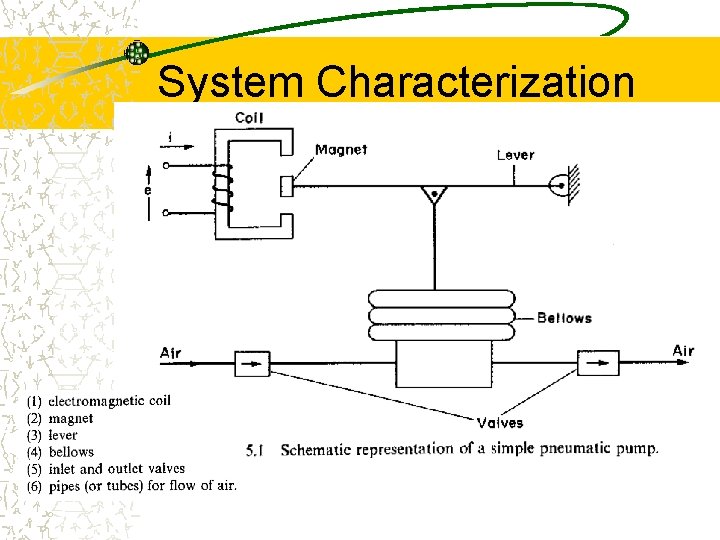
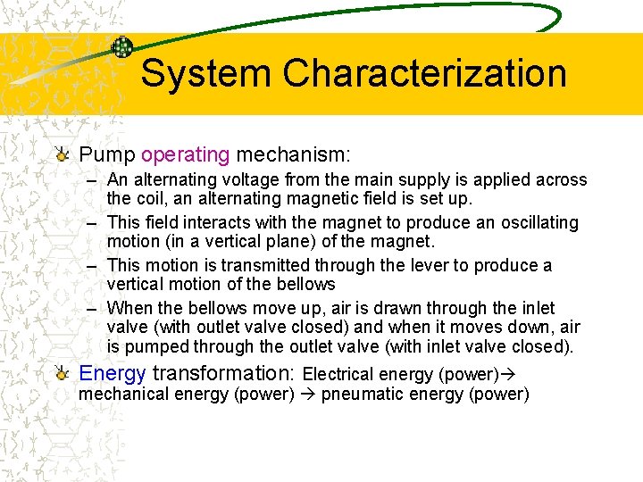
System Characterization Pump operating mechanism: – An alternating voltage from the main supply is applied across the coil, an alternating magnetic field is set up. – This field interacts with the magnet to produce an oscillating motion (in a vertical plane) of the magnet. – This motion is transmitted through the lever to produce a vertical motion of the bellows – When the bellows move up, air is drawn through the inlet valve (with outlet valve closed) and when it moves down, air is pumped through the outlet valve (with inlet valve closed). Energy transformation: Electrical energy (power) mechanical energy (power) pneumatic energy (power)

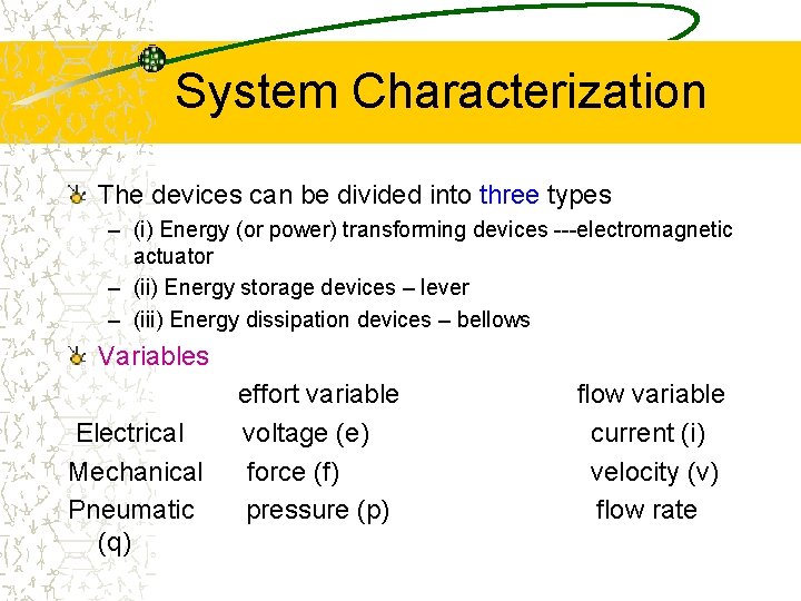
System Characterization The devices can be divided into three types – (i) Energy (or power) transforming devices ---electromagnetic actuator – (ii) Energy storage devices – lever – (iii) Energy dissipation devices – bellows Variables Electrical Mechanical Pneumatic (q) effort variable voltage (e) force (f) pressure (p) flow variable current (i) velocity (v) flow rate

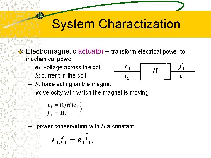
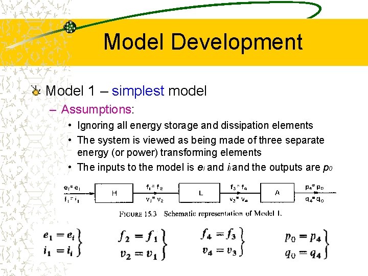
System Charactization Electromagnetic actuator – transform electrical power to mechanical power – e 1: voltage across the coil – i 1: current in the coil – f 1: force acting on the magnet – v 1: velocity with which the magnet is moving – power conservation with H a constant

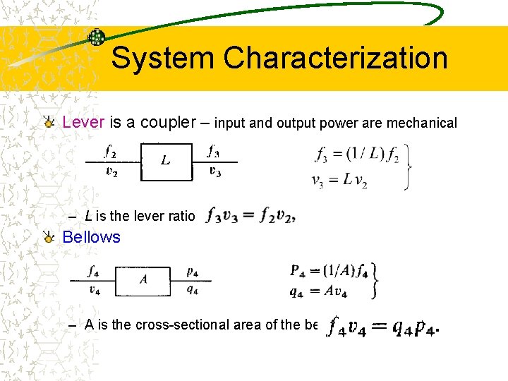
System Characterization Lever is a coupler – input and output power are mechanical – L is the lever ratio Bellows – A is the cross-sectional area of the bellows

Model Development Model 1 – simplest model – Assumptions: • Ignoring all energy storage and dissipation elements • The system is viewed as being made of three separate energy (or power) transforming elements • The inputs to the model is ei and ii and the outputs are p 0 and q 0.

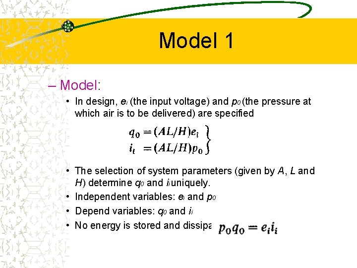
Model 1 – Model: • In design, ei (the input voltage) and p 0 (the pressure at which air is to be delivered) are specified • The selection of system parameters (given by A, L and H) determine q 0 and ii uniquely. • Independent variables: ei and p 0 • Depend variables: q 0 and ii • No energy is stored and dissipated:

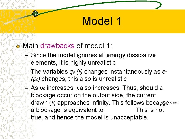
Model 1 Main drawbacks of model 1: – Since the model ignores all energy dissipative elements, it is highly unrealistic – The variables q 0 (ii) changes instantaneously as ei (p 0) changes, this also is unrealistic – As p 0 increases, ii also increases. Thus, should a blockage occur on the output side, the current drawn (ii) approaches infinity. This follows because a blockage is equivalent to This is not true, and hence the model is unacceptable.

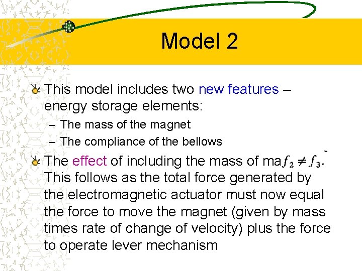
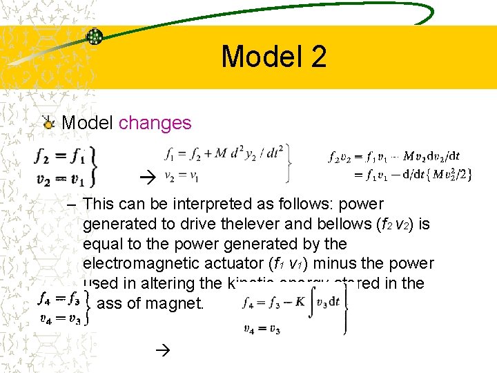
Model 2 This model includes two new features – energy storage elements: – The mass of the magnet – The compliance of the bellows The effect of including the mass of magnet is This follows as the total force generated by the electromagnetic actuator must now equal the force to move the magnet (given by mass times rate of change of velocity) plus the force to operate lever mechanism

Model 2 Model changes – This can be interpreted as follows: power generated to drive thelever and bellows (f 2 v 2) is equal to the power generated by the electromagnetic actuator (f 1 v 1) minus the power used in altering the kinetic energy stored in the mass of magnet.

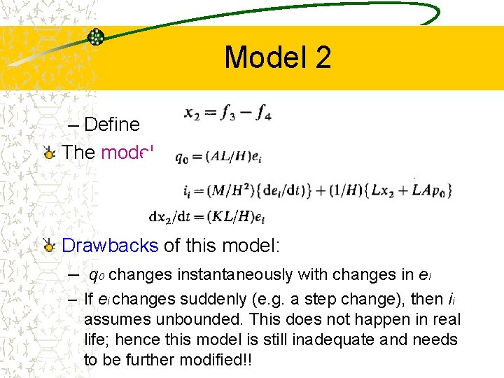
Model 2 – Define The model Drawbacks of this model: – q 0 changes instantaneously with changes in ei – If ei changes suddenly (e. g. a step change), then ii assumes unbounded. This does not happen in real life; hence this model is still inadequate and needs to be further modified!!

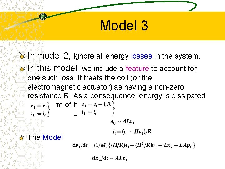
Model 3 In model 2, ignore all energy losses in the system. In this model, we include a feature to account for one such loss. It treats the coil (or the electromagnetic actuator) as having a non-zero resistance R. As a consequence, energy is dissipated in the form of heat. The Model

Model 3 This model overcomes all the drawbacks of model 1. However, it is still not adequate as it ignores various other features – compressibility, air friction, etc. The underlying mathematical formulation for both model 2 and 3 is the same in that they each involve two coupled ODEs. However, in model 1, the underlying formulation is algebraic!! In general, as we make the system characterization more detailed, i. e. include more features, the complexity of the underlying formulation use in the

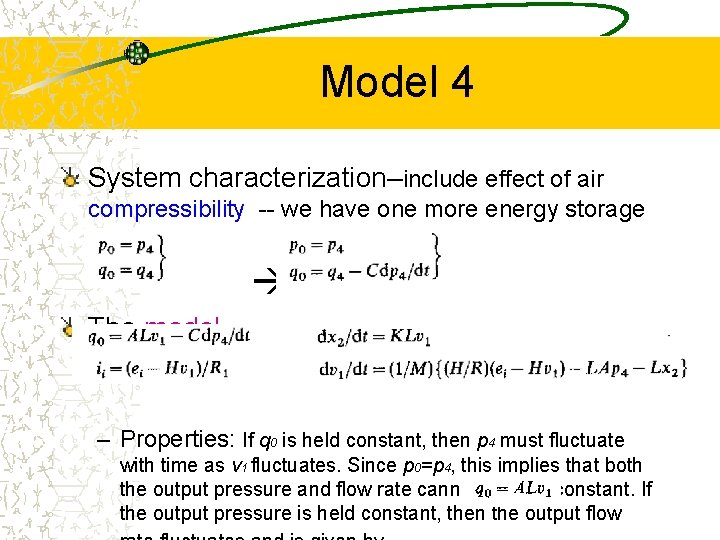
Model 4 System characterization–include effect of air compressibility -- we have one more energy storage element The model – Properties: If q 0 is held constant, then p 4 must fluctuate with time as v 1 fluctuates. Since p 0=p 4, this implies that both the output pressure and flow rate cannot be held constant. If the output pressure is held constant, then the output flow

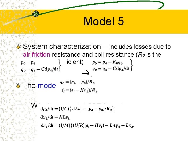
Model 5 System characterization – includes losses due to air friction resistance and coil resistance (R 0 is the resistance coefficient) The model – With (three coupled ODEs)

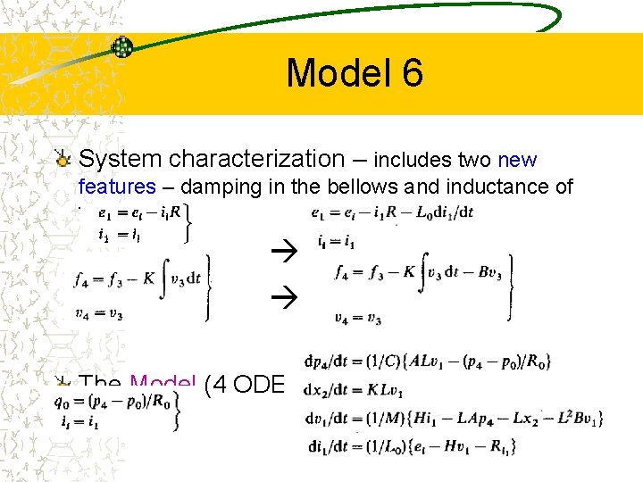
Model 6 System characterization – includes two new features – damping in the bellows and inductance of the coil The Model (4 ODEs)

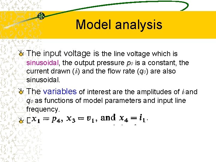
Model analysis The input voltage is the line voltage which is sinusoidal, the output pressure p 0 is a constant, the current drawn (ii) and the flow rate (q 0) are also sinusoidal. The variables of interest are the amplitudes of ii and q 0 as functions of model parameters and input line frequency. Define

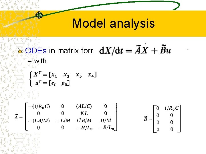
Model analysis ODEs in matrix form – with

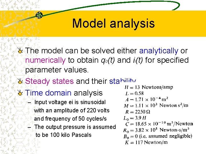
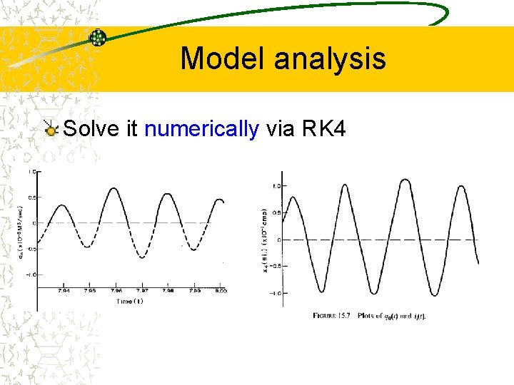
Model analysis The model can be solved either analytically or numerically to obtain q 0(t) and ii(t) for specified parameter values. Steady states and their stability Time domain analysis – Input voltage ei is sinusoidal with an amplitude of 220 volts and frequency of 50 cycles/s – The output pressure is assumed to be 100 kilo Pascals

Model analysis Solve it numerically via RK 4

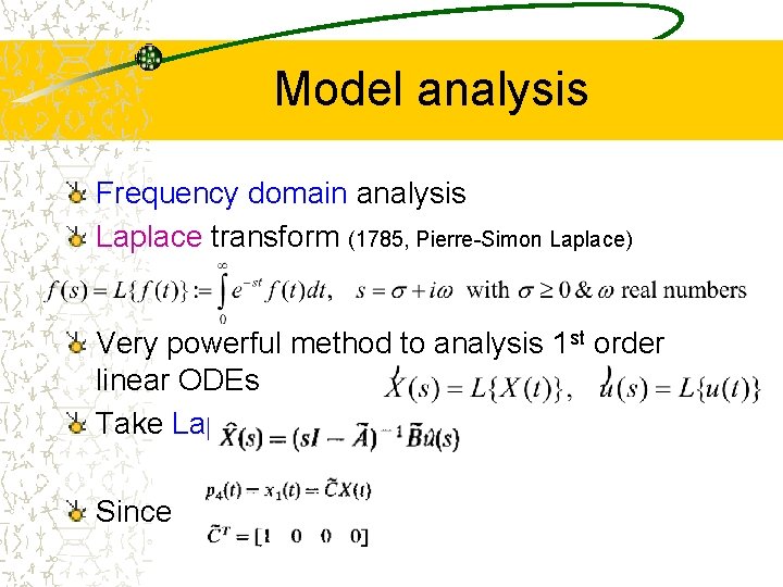
Model analysis Frequency domain analysis Laplace transform (1785, Pierre-Simon Laplace) Very powerful method to analysis 1 st order linear ODEs Take Laplace transform Since

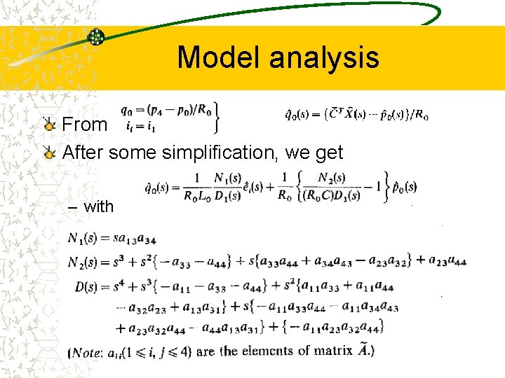
Model analysis From After some simplification, we get – with

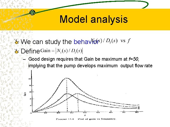
Model analysis We can study the behavior Define – Good design requires that Gain be maximum at f=50, implying that the pump develops maximum output flow rate f=50

Discussions and conclusions Discussions – From model 1 up to model 6, each model is an improvement over the previous one. Thus, models 1 -5 are special cases of model 6. – Model 1 uses a static formulation with only 3 parameters, model 6 uses a dynamic one with 4 coupled 1 st-order linear ODEs. – All the relationships are linear. Thus they are justified only when changes in the variables are small. When the changes become large, the linear relationships are no longer valid and one needs to use nonlinear relationships.

Conclusions A design problem where mathematical model plays an important role in the engineering task of designing. Further question is to transform the problem to an optimization problem by defining the optimization criterion as the maximization of Gain at f=50. Here we illustrate the iterative nature of model building: starting from the simplest model and increasing the complexity till an adequate model of least complexity is obtained!!