Improved Hough Transform We can then define the

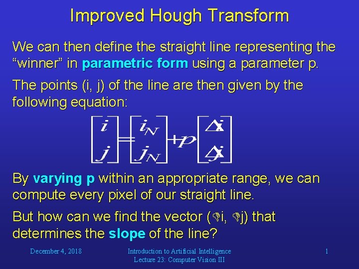
Improved Hough Transform We can then define the straight line representing the “winner” in parametric form using a parameter p. The points (i, j) of the line are then given by the following equation: By varying p within an appropriate range, we can compute every pixel of our straight line. But how can we find the vector ( i, j) that determines the slope of the line? December 4, 2018 Introduction to Artificial Intelligence Lecture 23: Computer Vision III 1

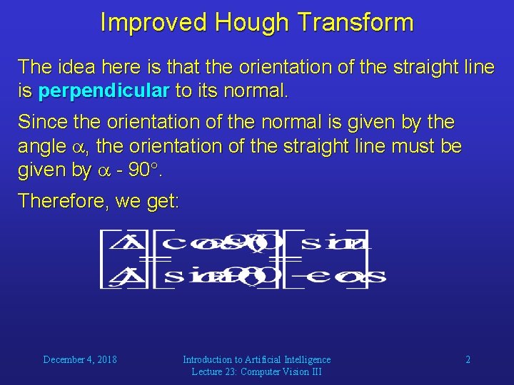
Improved Hough Transform The idea here is that the orientation of the straight line is perpendicular to its normal. Since the orientation of the normal is given by the angle , the orientation of the straight line must be given by - 90. Therefore, we get: December 4, 2018 Introduction to Artificial Intelligence Lecture 23: Computer Vision III 2

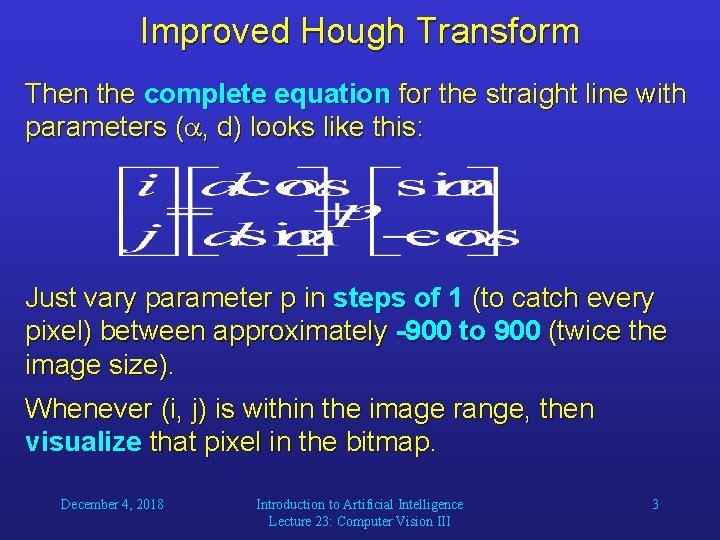
Improved Hough Transform Then the complete equation for the straight line with parameters ( , d) looks like this: Just vary parameter p in steps of 1 (to catch every pixel) between approximately -900 to 900 (twice the image size). Whenever (i, j) is within the image range, then visualize that pixel in the bitmap. December 4, 2018 Introduction to Artificial Intelligence Lecture 23: Computer Vision III 3

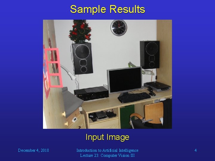
Sample Results Input Image December 4, 2018 Introduction to Artificial Intelligence Lecture 23: Computer Vision III 4

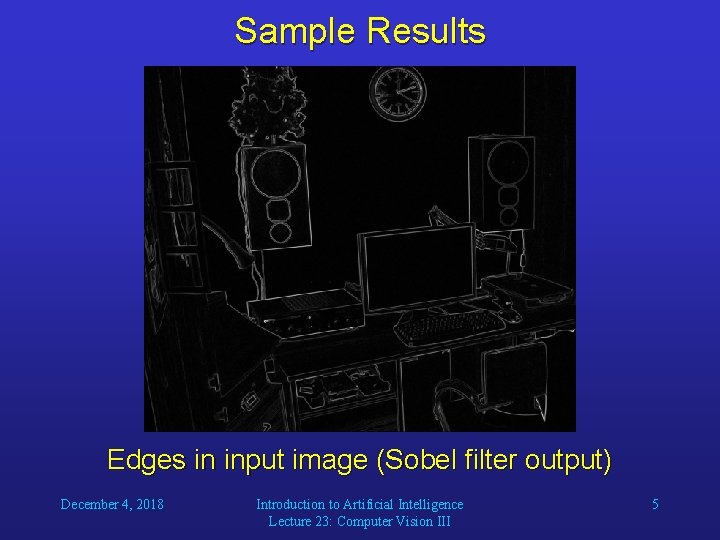
Sample Results Edges in input image (Sobel filter output) December 4, 2018 Introduction to Artificial Intelligence Lecture 23: Computer Vision III 5

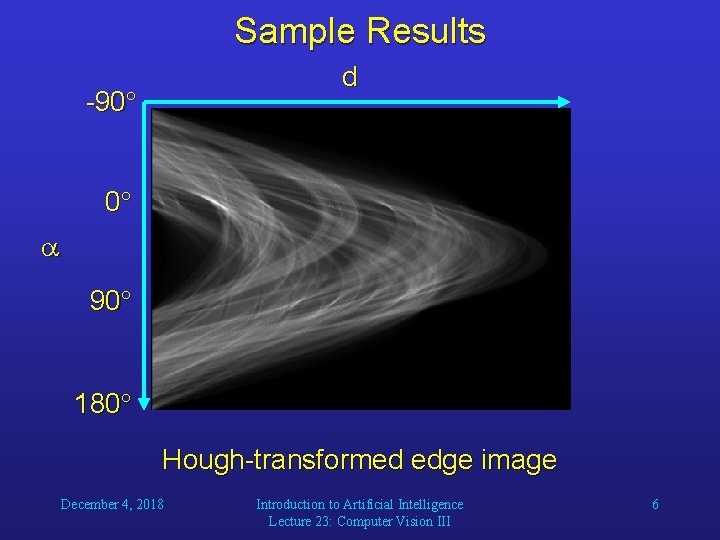
Sample Results d -90 0 90 180 Hough-transformed edge image December 4, 2018 Introduction to Artificial Intelligence Lecture 23: Computer Vision III 6

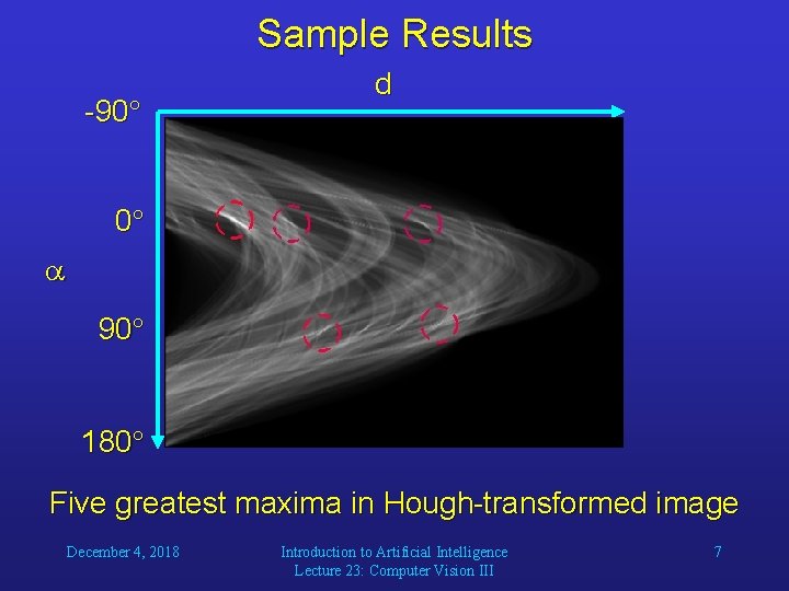
Sample Results -90 d 0 90 180 Five greatest maxima in Hough-transformed image December 4, 2018 Introduction to Artificial Intelligence Lecture 23: Computer Vision III 7

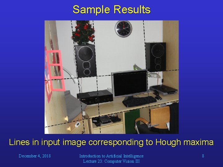
Sample Results Lines in input image corresponding to Hough maxima December 4, 2018 Introduction to Artificial Intelligence Lecture 23: Computer Vision III 8

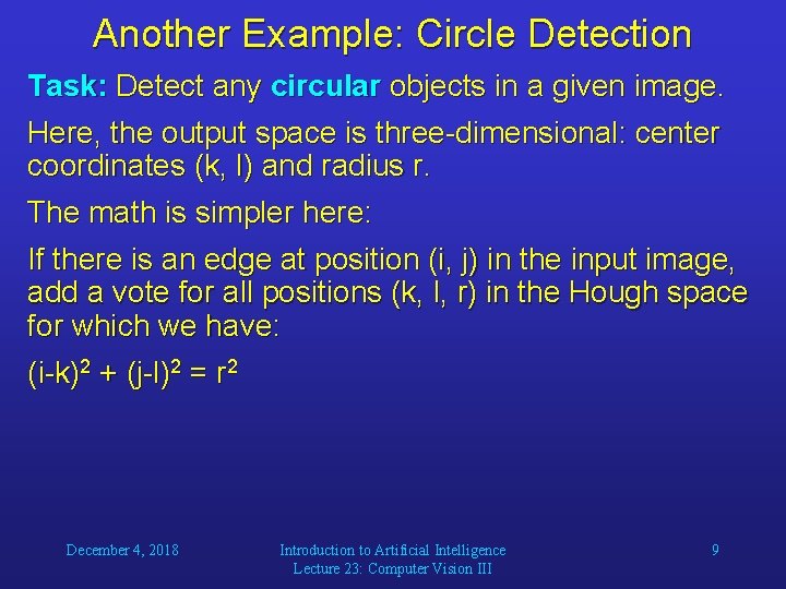
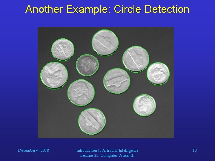
Another Example: Circle Detection Task: Detect any circular objects in a given image. Here, the output space is three-dimensional: center coordinates (k, l) and radius r. The math is simpler here: If there is an edge at position (i, j) in the input image, add a vote for all positions (k, l, r) in the Hough space for which we have: (i-k)2 + (j-l)2 = r 2 December 4, 2018 Introduction to Artificial Intelligence Lecture 23: Computer Vision III 9

Another Example: Circle Detection December 4, 2018 Introduction to Artificial Intelligence Lecture 23: Computer Vision III 10

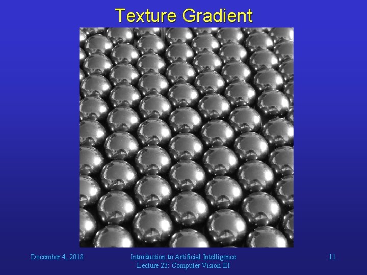
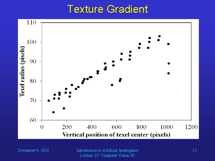
Texture Gradient December 4, 2018 Introduction to Artificial Intelligence Lecture 23: Computer Vision III 11

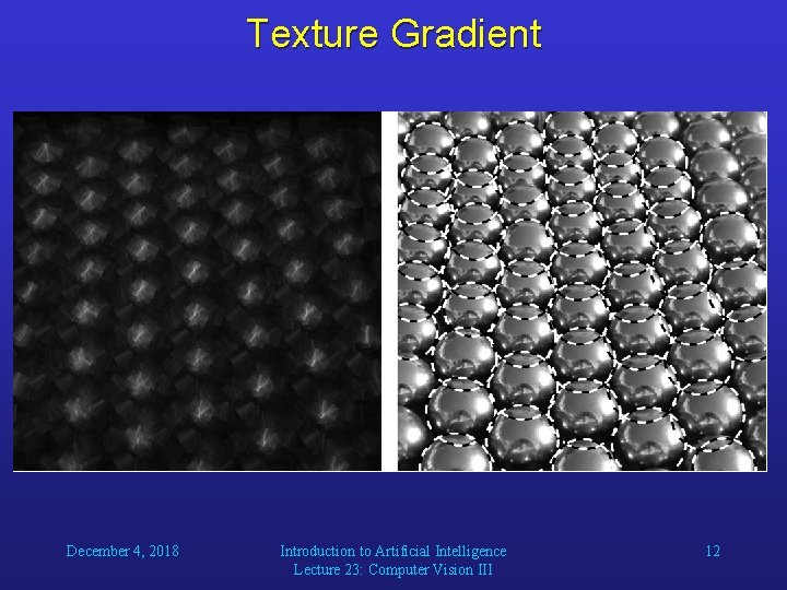
Texture Gradient December 4, 2018 Introduction to Artificial Intelligence Lecture 23: Computer Vision III 12

Texture Gradient December 4, 2018 Introduction to Artificial Intelligence Lecture 23: Computer Vision III 13

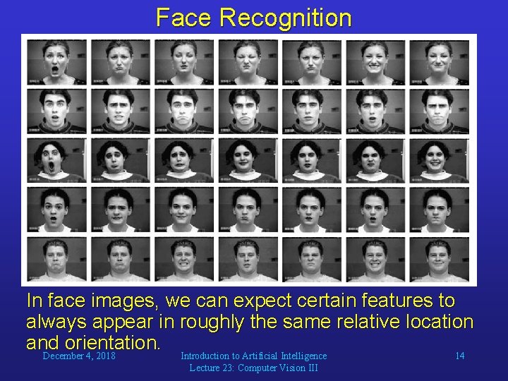
Face Recognition In face images, we can expect certain features to always appear in roughly the same relative location and orientation. December 4, 2018 Introduction to Artificial Intelligence 14 Lecture 23: Computer Vision III

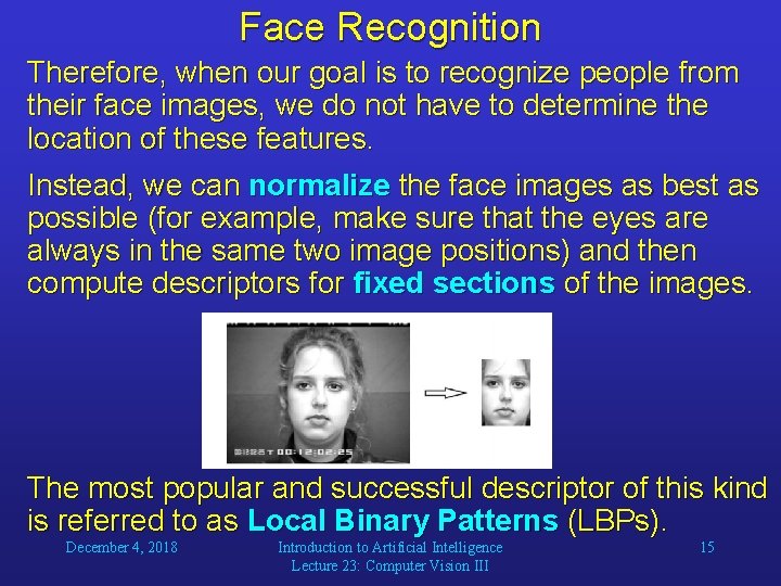
Face Recognition Therefore, when our goal is to recognize people from their face images, we do not have to determine the location of these features. Instead, we can normalize the face images as best as possible (for example, make sure that the eyes are always in the same two image positions) and then compute descriptors for fixed sections of the images. The most popular and successful descriptor of this kind is referred to as Local Binary Patterns (LBPs). December 4, 2018 Introduction to Artificial Intelligence Lecture 23: Computer Vision III 15

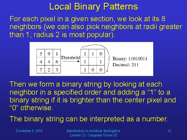
Local Binary Patterns For each pixel in a given section, we look at its 8 neighbors (we can also pick neighbors at radii greater than 1; radius 2 is most popular). Then we form a binary string by looking at each neighbor in a specified order and adding a “ 1” to a binary string if it is brighter than the center pixel and “ 0” otherwise. The binary string can be interpreted as a number. December 4, 2018 Introduction to Artificial Intelligence Lecture 23: Computer Vision III 16