Important Probability Distributions 2 Important named continuous probability
Important Probability Distributions 2 Important “named” continuous probability distributions that come up all the time
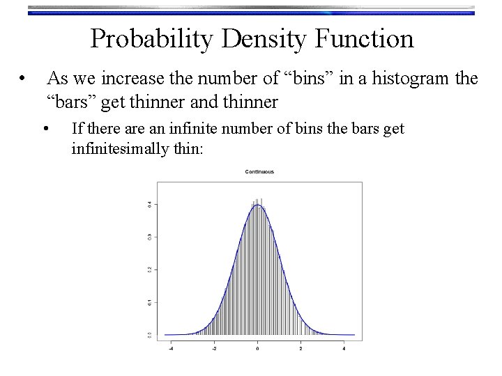
Probability Density Function • As we increase the number of “bins” in a histogram the “bars” get thinner and thinner • If there an infinite number of bins the bars get infinitesimally thin:
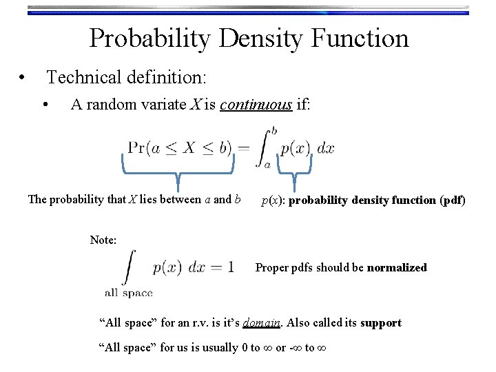
Probability Density Function • Technical definition: • A random variate X is continuous if: The probability that X lies between a and b p(x): probability density function (pdf) Note: Proper pdfs should be normalized “All space” for an r. v. is it’s domain. Also called its support “All space” for us is usually 0 to ∞ or -∞ to ∞
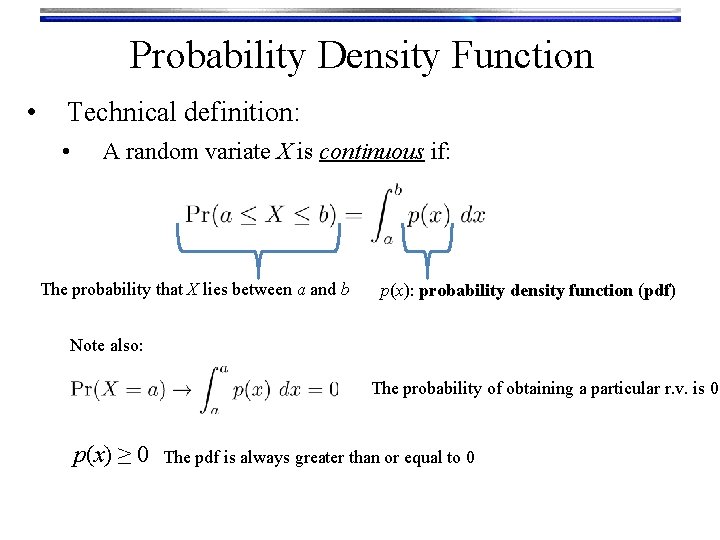
Probability Density Function • Technical definition: • A random variate X is continuous if: The probability that X lies between a and b p(x): probability density function (pdf) Note also: The probability of obtaining a particular r. v. is 0 p(x) ≥ 0 The pdf is always greater than or equal to 0
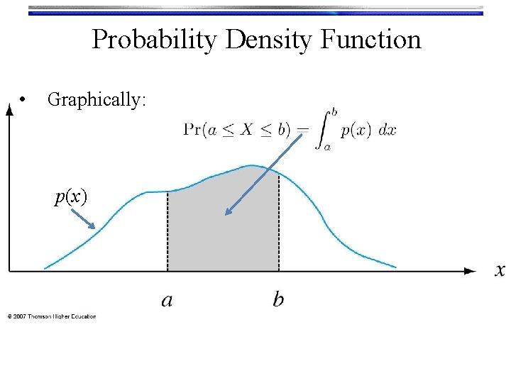
Probability Density Function • Graphically: p(x)
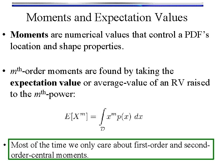
Moments and Expectation Values • Moments are numerical values that control a PDF’s location and shape properties. • mth-order moments are found by taking the expectation value or average-value of an RV raised to the mth-power: • Most of the time we only care about first-order and secondorder-central moments.
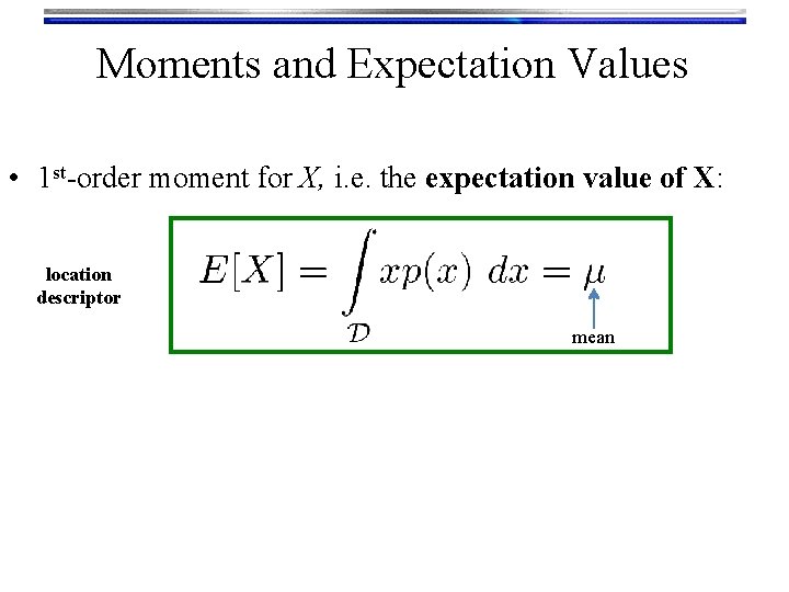
Moments and Expectation Values • 1 st-order moment for X, i. e. the expectation value of X: location descriptor mean
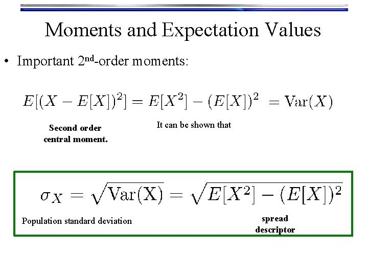
Moments and Expectation Values • Important 2 nd-order moments: Second order central moment. Population standard deviation It can be shown that spread descriptor
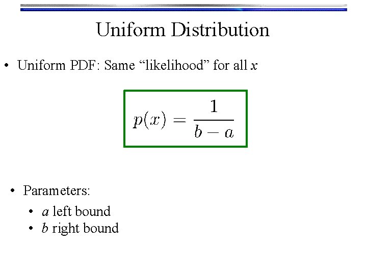
Uniform Distribution • Uniform PDF: Same “likelihood” for all x • Parameters: • a left bound • b right bound
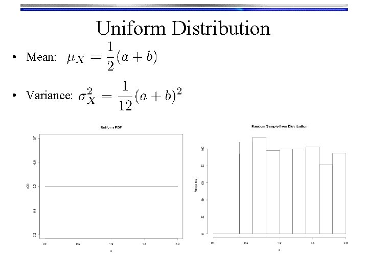
Uniform Distribution • Mean: • Variance:
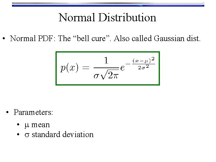
Normal Distribution • Normal PDF: The “bell cure”. Also called Gaussian dist. • Parameters: • m mean • s standard deviation
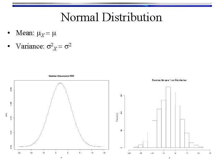
Normal Distribution • Mean: m. X = m • Variance: s 2 X = s 2
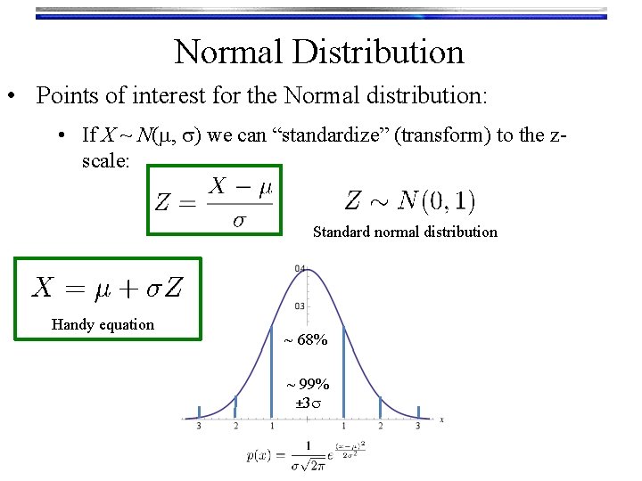
Normal Distribution • Points of interest for the Normal distribution: • If X ~ N(m, s) we can “standardize” (transform) to the zscale: Standard normal distribution Handy equation ~ 68% ~± 1 s 95% ~± 2 s 99% ± 3 s
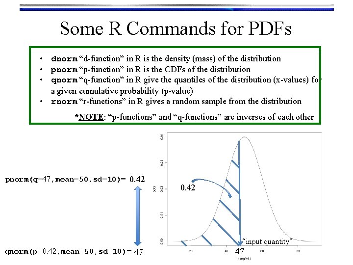
Some R Commands for PDFs • dnorm “d-function” in R is the density (mass) of the distribution • pnorm “p-function” in R is the CDFs of the distribution • qnorm “q-function” in R give the quantiles of the distribution (x-values) for a given cumulative probability (p-value) • rnorm “r-functions” in R gives a random sample from the distribution *NOTE: “p-functions” and “q-functions” are inverses of each other pnorm(q=47, mean=50, sd=10)= 0. 42 “input quantity” qnorm(p=0. 42, mean=50, sd=10)= 47 47
Example: quantiles/percentiles A sample of methamphetamine in blood certified reference material (CRM) is obtained as a standard for calibration of methodology in a tox lab. The concentration of the CRM is certified to follow a normal distribution with mean concentration of 50 ng/m. L and standard deviation of 10 ng/m. L. What maximum concentration can we expect for 90% of the samples we may measure?
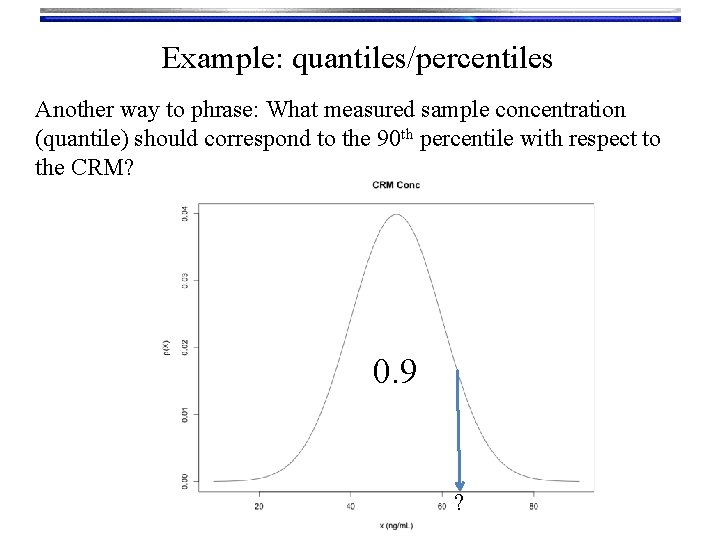
Example: quantiles/percentiles Another way to phrase: What measured sample concentration (quantile) should correspond to the 90 th percentile with respect to the CRM? 0. 9 ?
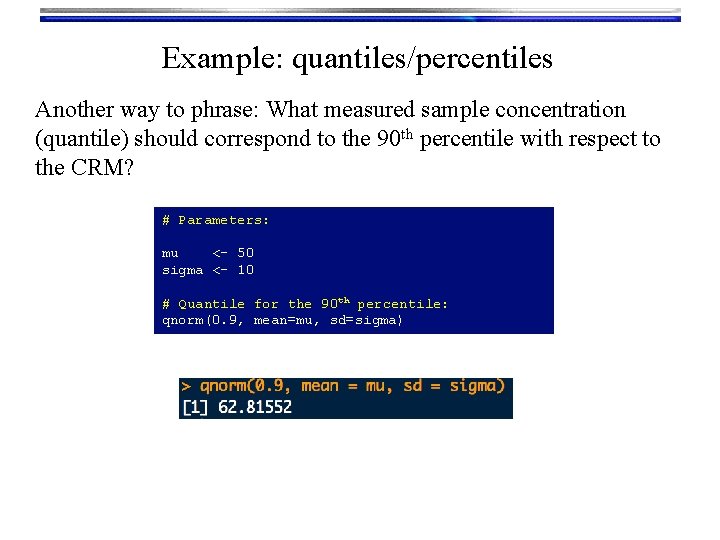
Example: quantiles/percentiles Another way to phrase: What measured sample concentration (quantile) should correspond to the 90 th percentile with respect to the CRM? # Parameters: mu <- 50 sigma <- 10 # Quantile for the 90 th percentile: qnorm(0. 9, mean=mu, sd=sigma)
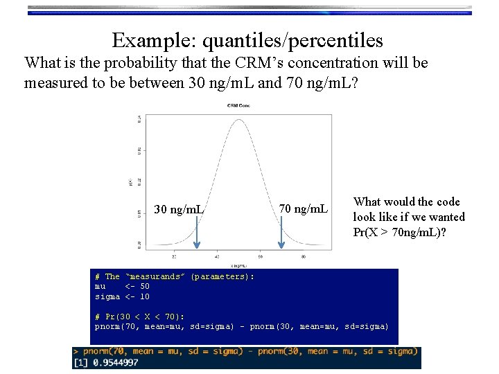
Example: quantiles/percentiles What is the probability that the CRM’s concentration will be measured to be between 30 ng/m. L and 70 ng/m. L? 30 ng/m. L 70 ng/m. L What would the code look like if we wanted Pr(X > 70 ng/m. L)? # The “measurands” (parameters): mu <- 50 sigma <- 10 # Pr(30 < X < 70): pnorm(70, mean=mu, sd=sigma) – pnorm(30, mean=mu, sd=sigma)
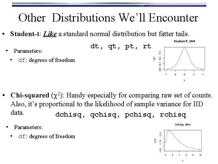
Other Distributions We’ll Encounter • Student-t: Like a standard normal distribution but fatter tails. • Parameters: • df: degrees of freedom dt, qt, pt, rt • Chi-squared (c 2): Handy especially for comparing raw set of counts. Also, it’s proportional to the likelihood of sample variance for IID data. dchisq, qchisq, pchisq, rchisq • Parameters: • df: degrees of freedom
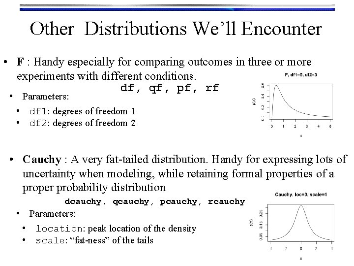
Other Distributions We’ll Encounter • F : Handy especially for comparing outcomes in three or more experiments with different conditions. df, qf, pf, rf • Parameters: • df 1: degrees of freedom 1 • df 2: degrees of freedom 2 • Cauchy : A very fat-tailed distribution. Handy for expressing lots of uncertainty when modeling, while retaining formal properties of a proper probability distribution dcauchy, qcauchy, pcauchy, rcauchy • Parameters: • location: peak location of the density • scale: “fat-ness” of the tails
- Slides: 20