Important Probability Distributions 2 Discrete Data Probability Mass

Important Probability Distributions 2 Discrete Data: Probability Mass Functions and Cumulative Mass Distributions

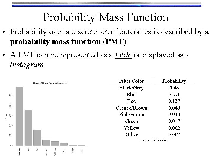
Probability Mass Function • Probability over a discrete set of outcomes is described by a probability mass function (PMF) • A PMF can be represented as a table or displayed as a histogram Fiber Color Black/Grey Blue Red Orange/Brown Pink/Purple Green Yellow Other Probability 0. 48 0. 291 0. 127 0. 048 0. 033 0. 017 0. 002 Data from dafs: fiber. color. df

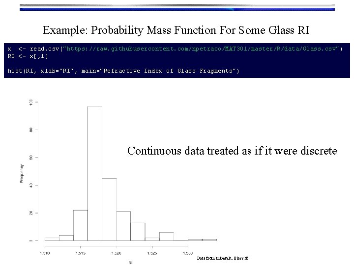
Example: Probability Mass Function For Some Glass RI x <- read. csv("https: //raw. githubusercontent. com/npetraco/MAT 301/master/R/data/Glass. csv") RI <- x[, 1] hist(RI, xlab="RI", main="Refractive Index of Glass Fragments") Continuous data treated as if it were discrete Data from mlbench: Glass. df

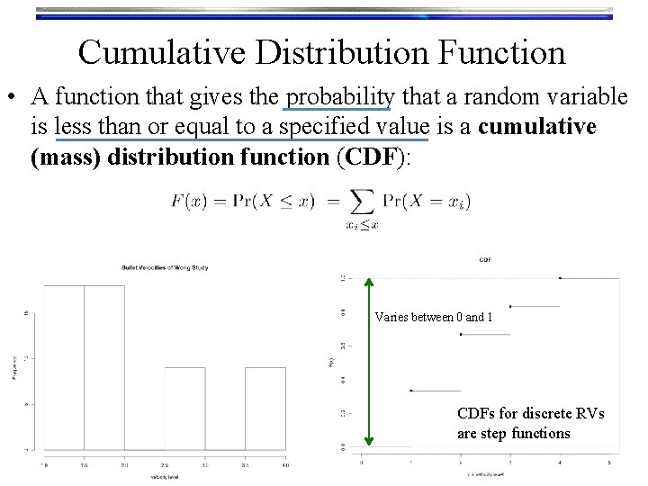
Cumulative Distribution Function • A function that gives the probability that a random variable is less than or equal to a specified value is a cumulative (mass) distribution function (CDF): Varies between 0 and 1 CDFs for discrete RVs are step functions

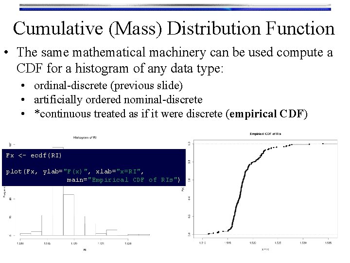
Cumulative (Mass) Distribution Function • The same mathematical machinery can be used compute a CDF for a histogram of any data type: • ordinal-discrete (previous slide) • artificially ordered nominal-discrete • *continuous treated as if it were discrete (empirical CDF) Fx <- ecdf(RI) plot(Fx, ylab="F(x)", xlab="x=RI", main="Empirical CDF of RIs")

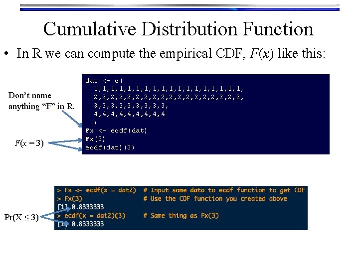
Cumulative Distribution Function • In R we can compute the empirical CDF, F(x) like this: Don’t name anything “F” in R. F(x = 3) Pr(X ≤ 3) dat <- c( 1, 1, 1, 1, 1, 2, 2, 2, 2, 2, 3, 3, 3, 4, 4, 4 ) Fx <- ecdf(dat) Fx(3) ecdf(dat)(3)

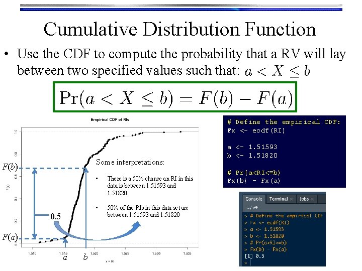
Cumulative Distribution Function • Use the CDF to compute the probability that a RV will lay between two specified values such that: # Define the empirical CDF: Fx <- ecdf(RI) Some interpretations: F(b) 0. 5 F(a) a b • There is a 50% chance an RI in this data is between 1. 51593 and 1. 51820 • 50% of the RIs in this data set are between 1. 51593 and 1. 51820 a <- 1. 51593 b <- 1. 51820 # Pr(a<RI<=b) Fx(b) - Fx(a)