Implicit Geometry Graham Rhodes Applied Research Associates Inc

Implicit Geometry Graham Rhodes Applied Research Associates, Inc.

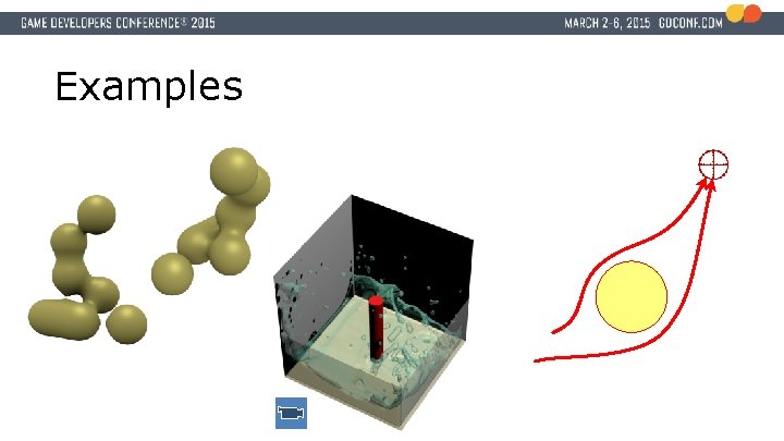
Examples

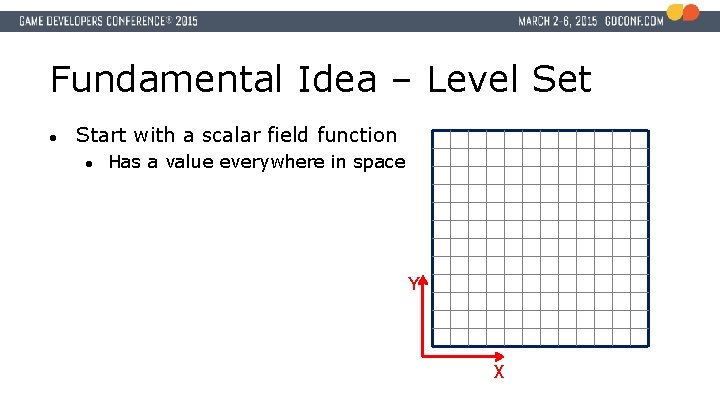
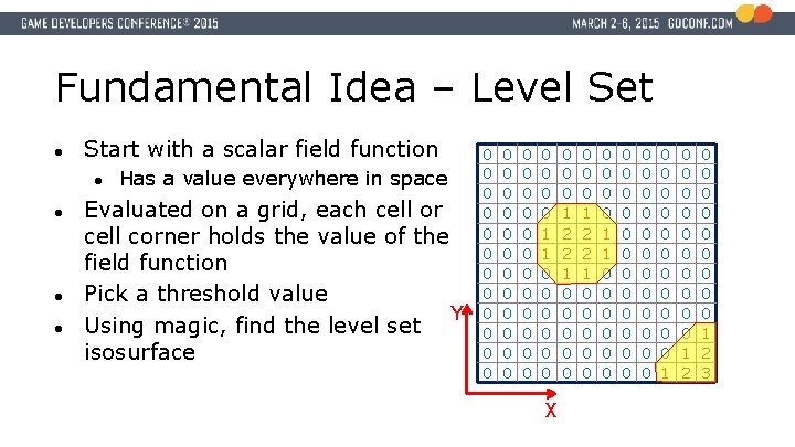
Fundamental Idea – Level Set ● Start with a scalar field function ● Has a value everywhere in space Y X

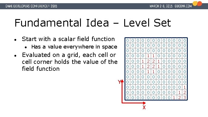
Fundamental Idea – Level Set ● Start with a scalar field function ● ● Has a value everywhere in space Evaluated on a grid, each cell or cell corner holds the value of the field function Y 0 0 0 0 0 0 0 0 0 0 1 1 0 0 0 X 0 0 0 1 2 2 1 0 0 0 0 1 1 0 0 0 0 0 0 0 0 0 0 0 1 0 0 0 0 0 1 2 3

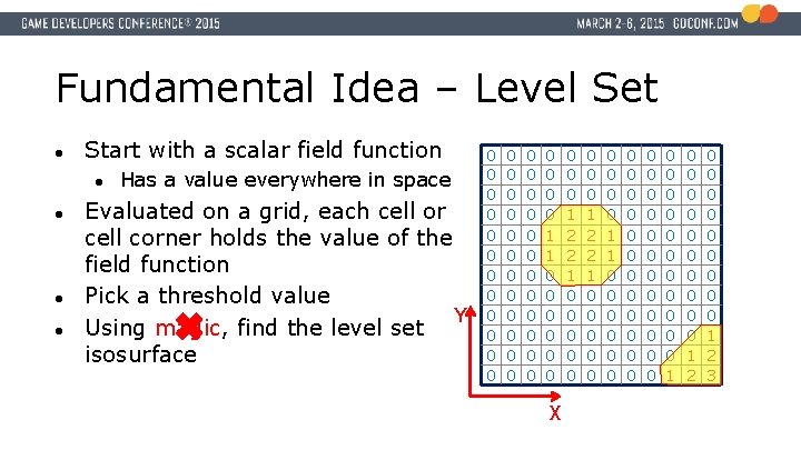
Fundamental Idea – Level Set ● Start with a scalar field function ● ● Has a value everywhere in space Evaluated on a grid, each cell or cell corner holds the value of the field function Pick a threshold value Y Using magic, find the level set isosurface 0 0 0 0 0 0 0 0 0 0 1 1 0 0 0 X 0 0 0 1 2 2 1 0 0 0 0 1 1 0 0 0 0 0 0 0 0 0 0 0 1 0 0 0 0 0 1 2 3

Fundamental Idea – Level Set ● Start with a scalar field function ● ● Has a value everywhere in space Evaluated on a grid, each cell or cell corner holds the value of the field function Pick a threshold value Y Using magic, find the level set isosurface 0 0 0 0 0 0 0 0 0 0 1 1 0 0 0 X 0 0 0 1 2 2 1 0 0 0 0 1 1 0 0 0 0 0 0 0 0 0 0 0 1 0 0 0 0 0 1 2 3

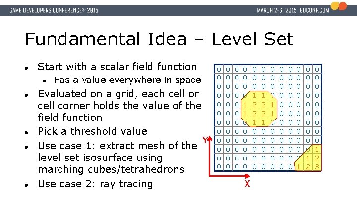
Fundamental Idea – Level Set ● Start with a scalar field function ● ● ● Has a value everywhere in space Evaluated on a grid, each cell or cell corner holds the value of the field function Pick a threshold value Y Use case 1: extract mesh of the level set isosurface using marching cubes/tetrahedrons Use case 2: ray tracing 0 0 0 0 0 0 0 0 0 0 1 1 0 0 0 X 0 0 0 1 2 2 1 0 0 0 0 1 1 0 0 0 0 0 0 0 0 0 0 0 1 0 0 0 0 0 1 2 3

I’m Interested In Modeling With Implicit Functions ● ● ● Surfaces Containment volumes and light fields Animation Paths

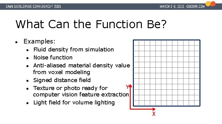
What Can the Function Be? ● Examples: ● ● ● Fluid density from simulation Noise function Anti-aliased material density value from voxel modeling Signed distance field Y Texture or photo ready for computer vision feature extraction Light field for volume lighting X

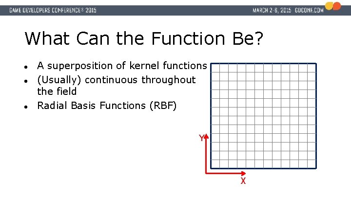
What Can the Function Be? ● ● ● A superposition of kernel functions (Usually) continuous throughout the field Radial Basis Functions (RBF) Y X

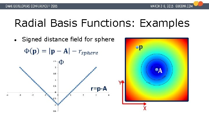
Radial Basis Functions: Examples ● Signed distance field for sphere r=p-A Y X

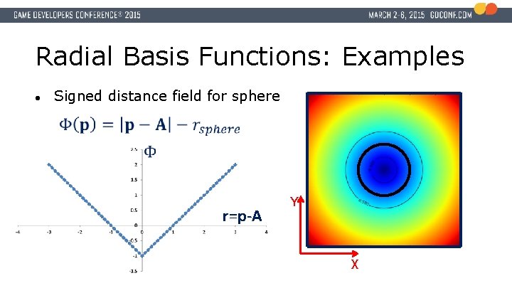
Radial Basis Functions: Examples ● Signed distance field for sphere r=p-A Y X

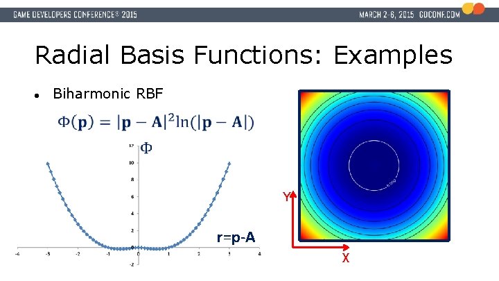
Radial Basis Functions: Examples ● Biharmonic RBF Y r=p-A X

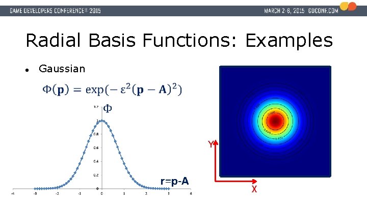
Radial Basis Functions: Examples ● Gaussian Y r=p-A X

Radial Basis Functions: Selection ● ● ● There are many other choices Choice of function depends on use case An important characteristic is the nature of the “support” of the RBF of choice ● ● Compact or finite Non-compact or infinite

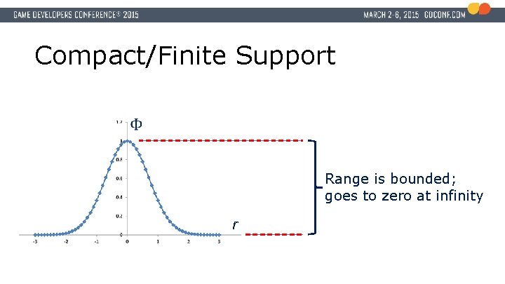
Compact/Finite Support Range is bounded; goes to zero at infinity r

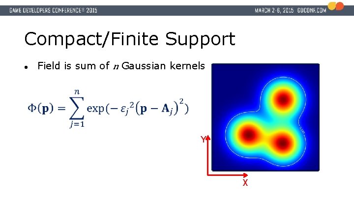
Compact/Finite Support ● Field is sum of n Gaussian kernels Y X

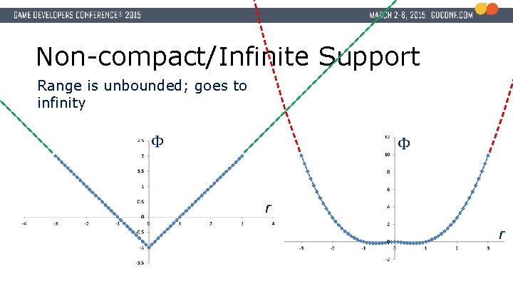
Non-compact/Infinite Support Range is unbounded; goes to infinity r r

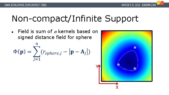
Non-compact/Infinite Support ● Field is sum of n kernels based on signed distance field for sphere Y X

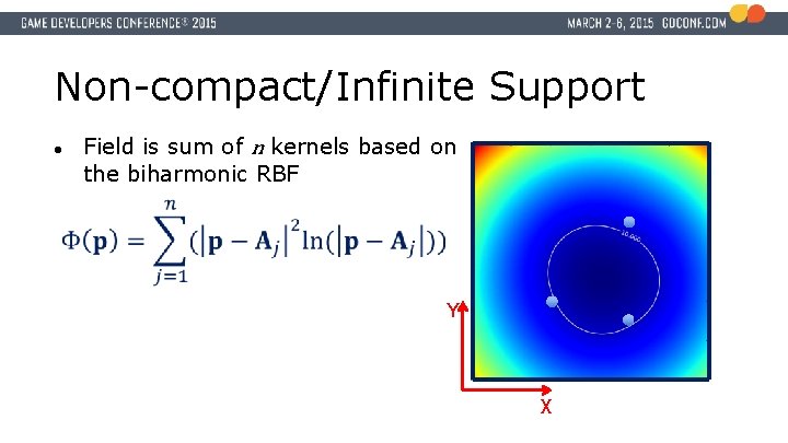
Non-compact/Infinite Support ● Field is sum of n kernels based on the biharmonic RBF Y X

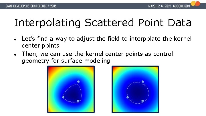
Interpolating Scattered Point Data ● ● Let’s find a way to adjust the field to interpolate the kernel center points Then, we can use the kernel center points as control geometry for surface modeling

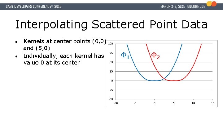
Interpolating Scattered Point Data ● ● Kernels at center points (0, 0) and (5, 0) Individually, each kernel has value 0 at its center

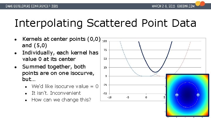
Interpolating Scattered Point Data ● ● ● Kernels at center points (0, 0) and (5, 0) Individually, each kernel has value 0 at its center Summed together, both points are on one isocurve, but… ● ● ● We’d like isocurve value = 0 It isn’t. Inconvenient How can we change this?

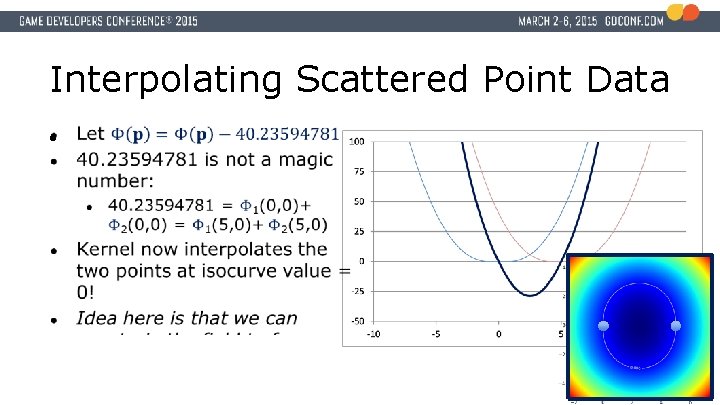
Interpolating Scattered Point Data ●

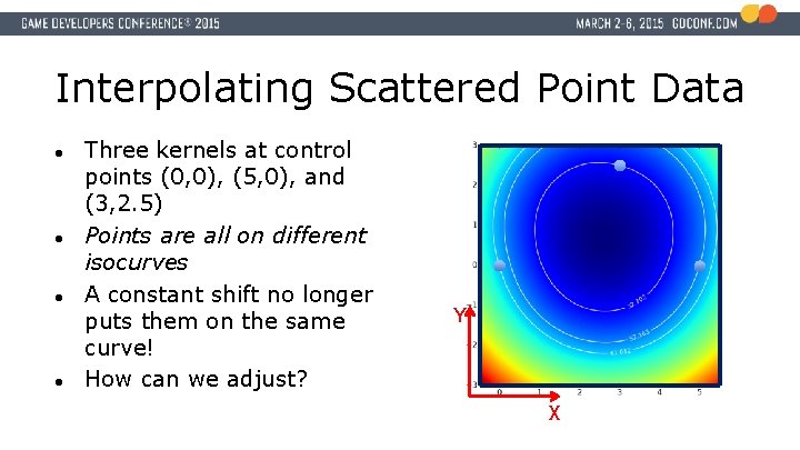
Interpolating Scattered Point Data ● ● Three kernels at control points (0, 0), (5, 0), and (3, 2. 5) Points are all on different isocurves A constant shift no longer puts them on the same curve! How can we adjust? Y X

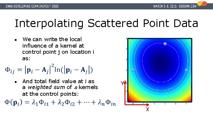
Interpolating Scattered Point Data ● We can write the local influence of a kernel at control point j on location i as: ● And total field value at i as a weighted sum of n kernels at the control points: Y X

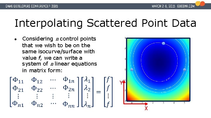
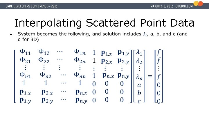
Interpolating Scattered Point Data ● Considering n control points that we wish to be on the same isocurve/surface with value f, we can write a system of n linear equations in matrix form: Y X

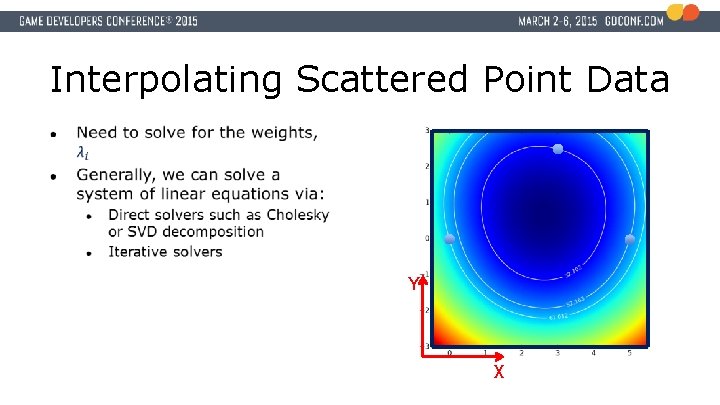
Interpolating Scattered Point Data Y X

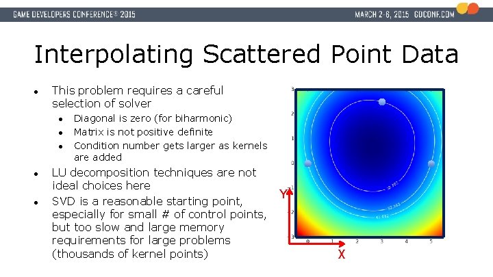
Interpolating Scattered Point Data ● This problem requires a careful selection of solver ● ● ● Diagonal is zero (for biharmonic) Matrix is not positive definite Condition number gets larger as kernels are added LU decomposition techniques are not ideal choices here Y SVD is a reasonable starting point, especially for small # of control points, but too slow and large memory requirements for large problems (thousands of kernel points) X

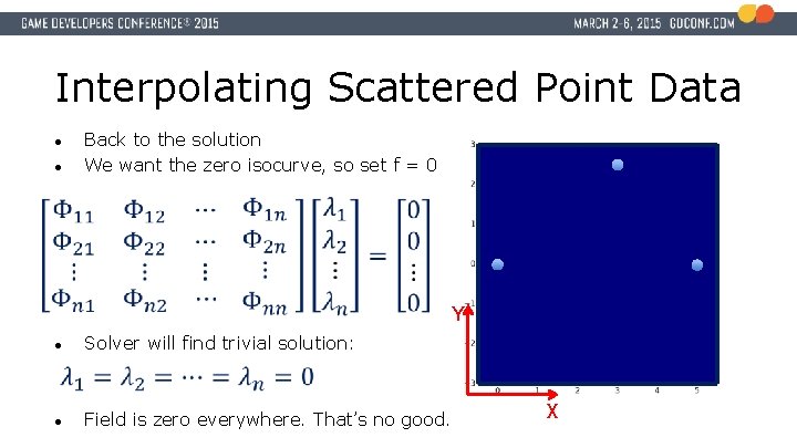
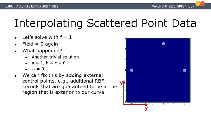
Interpolating Scattered Point Data ● ● Back to the solution We want the zero isocurve, so set f = 0 Y ● Solver will find trivial solution: ● Field is zero everywhere. That’s no good. X

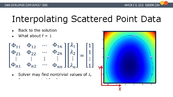
Interpolating Scattered Point Data Y X

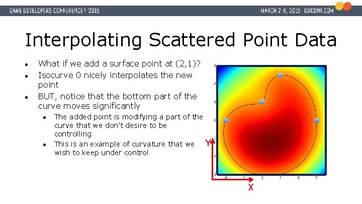
Interpolating Scattered Point Data ● ● ● What if we add a surface point at (2, 1)? Isocurve 0 nicely interpolates the new point BUT, notice that the bottom part of the curve moves significantly ● ● The added point is modifying a part of the curve that we don’t desire to be controlling This is an example of curvature that we Y wish to keep under control X

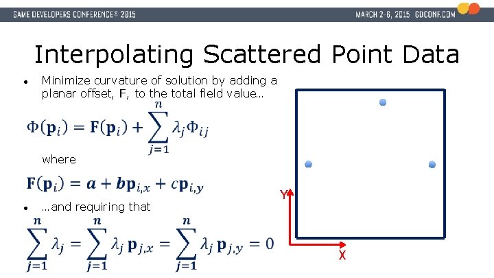
Interpolating Scattered Point Data ● Minimize curvature of solution by adding a planar offset, F, to the total field value… where ● …and requiring that Y X

Interpolating Scattered Point Data

Interpolating Scattered Point Data Y X

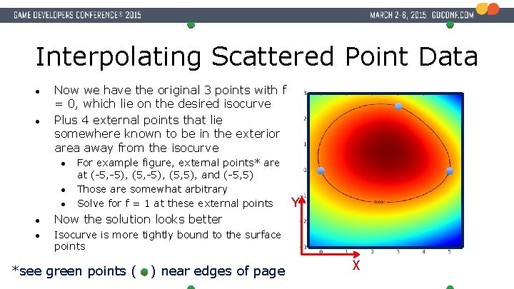
Interpolating Scattered Point Data ● ● Now we have the original 3 points with f = 0, which lie on the desired isocurve Plus 4 external points that lie somewhere known to be in the exterior area away from the isocurve ● ● ● For example figure, external points* are at (-5, -5), (5, 5), and (-5, 5) Those are somewhat arbitrary Solve for f = 1 at these external points ● Now the solution looks better ● Isocurve is more tightly bound to the surface points *see green points ( ) near edges of page Y X

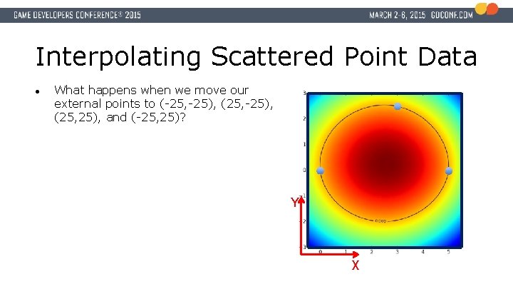
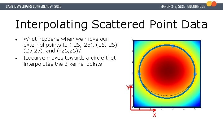
Interpolating Scattered Point Data ● What happens when we move our external points to (-25, -25), (25, -25), (25, 25), and (-25, 25)? Y X

Interpolating Scattered Point Data ● ● What happens when we move our external points to (-25, -25), (25, -25), (25, 25), and (-25, 25)? Isocurve moves towards a circle that interpolates the 3 kernel points Y X

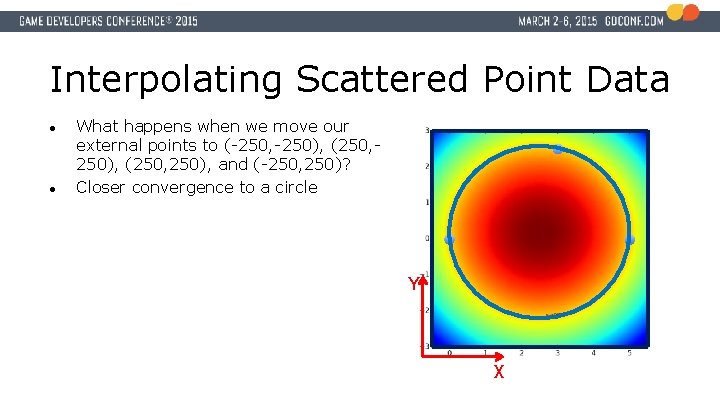
Interpolating Scattered Point Data ● ● What happens when we move our external points to (-250, -250), (250, 250), and (-250, 250)? Closer convergence to a circle Y X

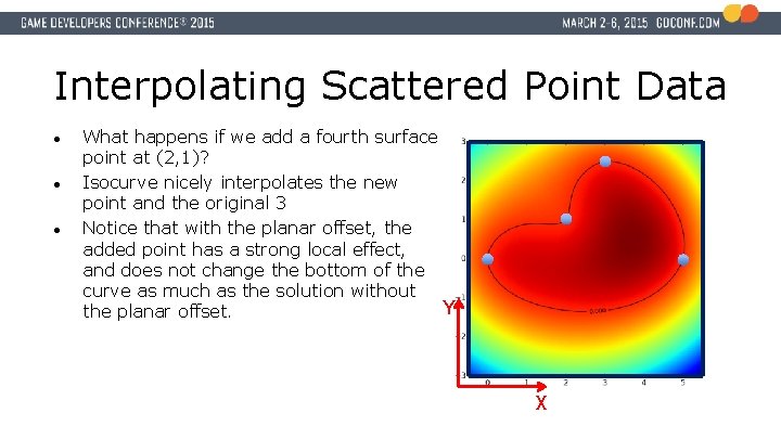
Interpolating Scattered Point Data ● ● ● What happens if we add a fourth surface point at (2, 1)? Isocurve nicely interpolates the new point and the original 3 Notice that with the planar offset, the added point has a strong local effect, and does not change the bottom of the curve as much as the solution without Y the planar offset. X

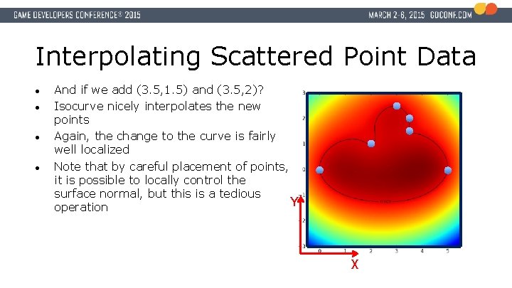
Interpolating Scattered Point Data ● ● And if we add (3. 5, 1. 5) and (3. 5, 2)? Isocurve nicely interpolates the new points Again, the change to the curve is fairly well localized Note that by careful placement of points, it is possible to locally control the surface normal, but this is a tedious Y operation X

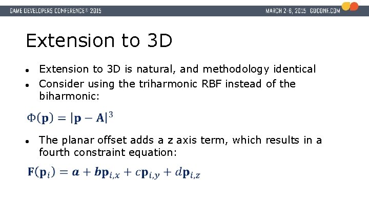
Extension to 3 D ● ● Extension to 3 D is natural, and methodology identical Consider using the triharmonic RBF instead of the biharmonic: ● The planar offset adds a z axis term, which results in a fourth constraint equation:

Takeaways ● ● ● Radial basis functions (RBF’s) and other kernel functions can be used to interpolate/extrapolate volumetric scalar field functions given scattered control points Choice of RBF depends on application, and is a function of compact vs. non -compact support Especially for RBF’s with non-compact support, a solver that is tolerant of non-positive definite matrices is required to solve for the RBF weight factors

Takeaways ● Example applications of RBF-based volumetric field and implicit surface modeling in games ● ● ● Light field modeling for volumetric lighting Generate polygon mesh for fluid rendering Use gradient of scalar field to generate animation or navigation paths

References ● ● ● Witkin, Andrew P. , and Paul S. Heckbert, “Using Particles to Sample and Control Implicit Surfaces, ” SIGGRAPH 1994 Turk, Greg, and James F. O’Brien, “Modeling with Implicit Surfaces that Interpolate, ” ACM Transactions in Graphics, Volume 21, Number 4, October 2002 Funkhouser, Thomas, “Implicit Surfaces, ” Princeton University, Fall 1999 (available on the Internet as PDF)

Contact ● Graham Rhodes ● grhodes@nc. rr. com

Appendix: An Incomplete/Failed Experiment in Modeling Curves/Surfaces with Simple Potential Flow Kernels

Modeling Implicit Surfaces using Fluid Flow ● ● When I presented this talk at GDC 2015, I spent some time attempting to explain an unfinished experiment Initial results of the experiment were unfortunately not promising Idea was to choose a basis function from classical potential field techniques that are historically used to simulate incompressible, irrotational fluid flow, e. g. , in the preliminary design of wings, airplanes, etc. What follows is the original GDC slides plus one additional introductory slide to explain my motivation

Modeling Implicit Surfaces using Fluid Flow ● ● I was motivated to experimental with potential flow kernels in part because of my personal background in computational fluid dynamics and airplane design (years ago) I believed that the potential flow kernels might offer true benefits for geometric surface modeling, for the following reason: ● ● ● Closed form equations exist for potential flow kernels based on linear and polygonal control geometry Such edge and surface-based kernels may provide better control over local surface properties Due to the basis in physics-based governing equations, gradient curves extracted from potential flow fields might be more pleasing than gradient curves extracted from other scalar fields

Modeling Implicit Surfaces using Fluid Flow ● ● I still believe that some interesting results can be obtained by using the linear and polygonal 2 D and 3 D kernels for potential fluid flow However, now I am convinced there would be no realized benefit since the cost of the linear and polygonal kernels is computationally too expensive, at least for evaluation at runtime in a game

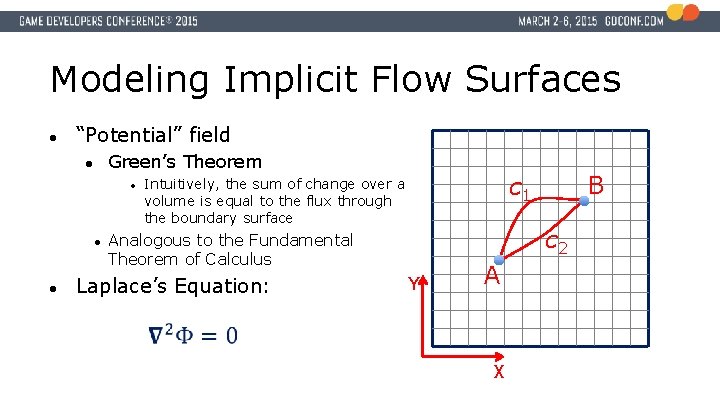
Modeling Implicit Flow Surfaces ● “Potential” field Green’s Theorem ● ● Analogous to the Fundamental Theorem of Calculus Laplace’s Equation: Y B c 1 Intuitively, the sum of change over a volume is equal to the flux through the boundary surface c 2 A X

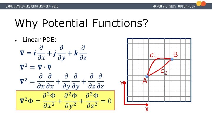
Why Potential Functions? Linear PDE: ● B c 1 c 2 Y A X

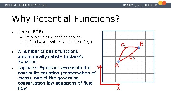
Why Potential Functions? ● Linear PDE: ● ● Principle of superposition applies If f and g are both solutions, then f+g is also a solution A number of basis functions automatically satisfy Laplace’s Equation represents the Y continuity equation (conservation of mass), one of the governing conservation law equations of fluid flow B c 1 c 2 A X

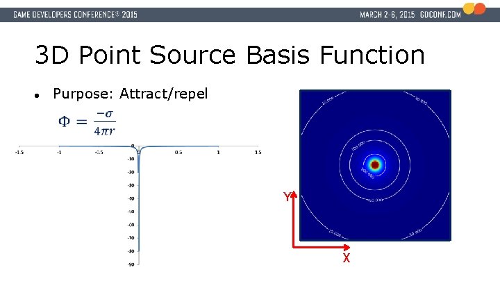
3 D Point Source Basis Function ● Purpose: Attract/repel Y X

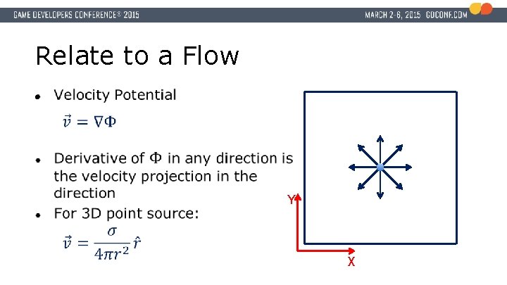
Relate to a Flow ● Y X

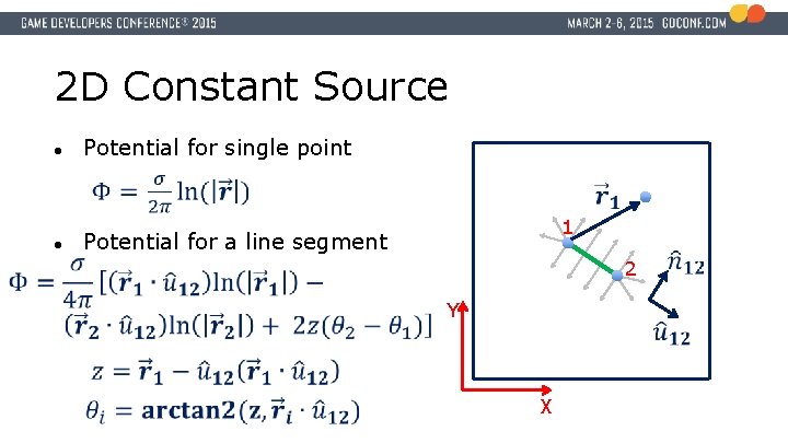
2 D Constant Source ● Potential for single point ● 1 Potential for a line segment 2 Y X

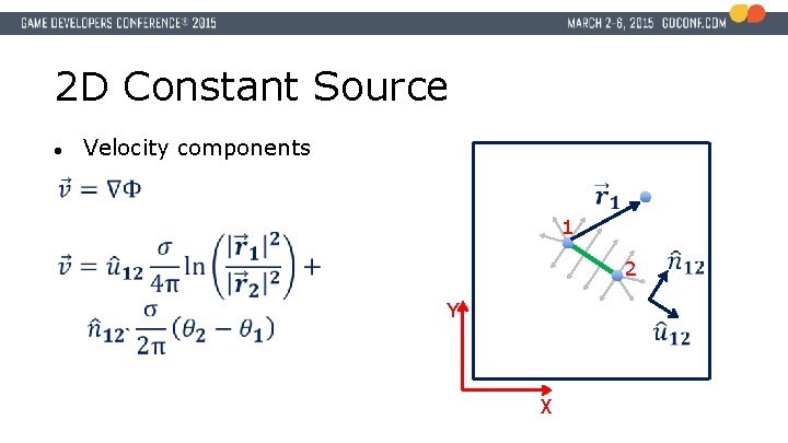
2 D Constant Source ● Velocity components 1 2 Y X

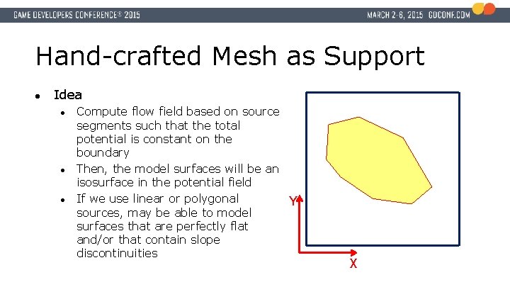
Hand-crafted Mesh as Support ● Idea ● ● ● Compute flow field based on source segments such that the total potential is constant on the boundary Then, the model surfaces will be an isosurface in the potential field If we use linear or polygonal Y sources, may be able to model surfaces that are perfectly flat and/or that contain slope discontinuities X

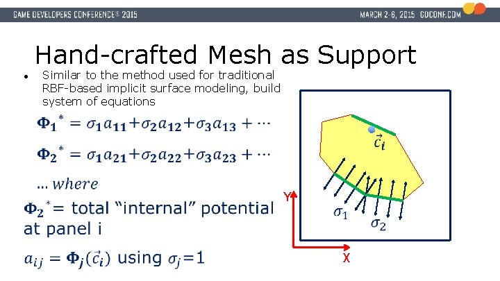
Hand-crafted Mesh as Support Similar to the method used for traditional RBF-based implicit surface modeling, build system of equations ● Y X

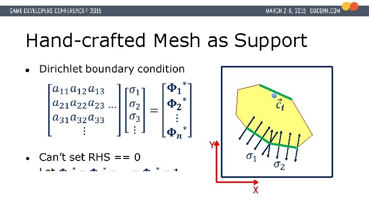
Hand-crafted Mesh as Support ● Y X

Evaluating the surface ● Once the source strengths are known ● ● Entire field can be evaluated at all points in space Evaluate directly, as needed, or sample into a grid for polygonalization

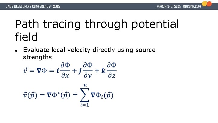
Path tracing through potential field ● Evaluate local velocity directly using source strengths

Superimpose other control kernels ● Crowd path finding ● ● Add a free stream to generate a field for entities moving in a general direction Add point source/sink for entities with specific targeting goals

Attention to speed ● Accelerating computation of potential ● ● Delegate to GPU Use far field solution Use approximate functions Take advantage of similarity ● ● Bake function into texture Evaluate by texture lookup + transform

Additional Takeaways ● ● ● The potential flow basis functions that are based on linear and polygonal control geometry may be beneficial for modeling implicit surfaces with difficult features such as perfectly flat regions and surface discontinuities The cost of computing these basis functions makes them unlikely candidates for use at runtime in a game; however, they may be useful in digital content creation tools The curves (e. g. , streamlines, pathlines) extracted using the velocity potential are consistent with physically based incompressible, irrotational fluid flows. ● ● The physical nature of these curves is useful for engineering applications, but may not be particularly beneficial for games The technique of using the gradient of the potential field to extract curves is not unique to the potential flow kernels. The gradient technique can be used with any scalar field. Any RBF-based field could produce interesting results.

Additional References ● Katz, Joseph, and Allen Plotkin, “Low-speed Aerodynamics: From Wing Theory to Panel Methods”