Imperfect Competition Pure Monopoly Price Average Revenue Quantity

Imperfect Competition Pure Monopoly

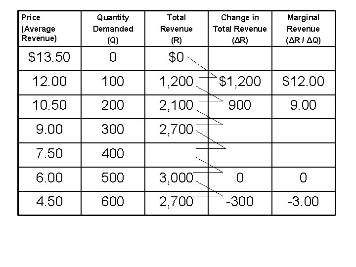
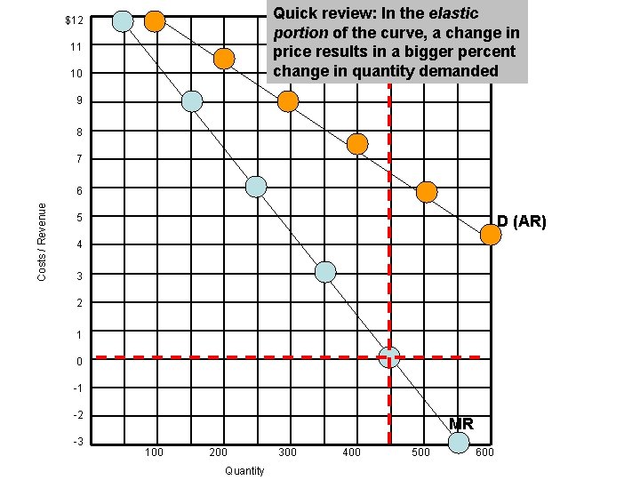
Price (Average Revenue) Quantity Demanded (Q) Total Revenue (R) Change in Total Revenue (ΔR) Marginal Revenue (ΔR / ΔQ) $13. 50 0 $0 12. 00 1, 200 $12. 00 10. 50 200 2, 100 9. 00 300 2, 700 7. 50 400 6. 00 500 3, 000 0 0 4. 50 600 2, 700 -3. 00

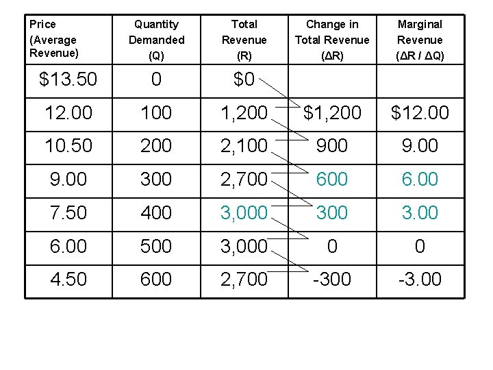
Price (Average Revenue) Quantity Demanded (Q) Total Revenue (R) Change in Total Revenue (ΔR) Marginal Revenue (ΔR / ΔQ) $13. 50 0 $0 12. 00 1, 200 $12. 00 10. 50 200 2, 100 9. 00 300 2, 700 6. 00 7. 50 400 3, 000 3. 00 6. 00 500 3, 000 0 0 4. 50 600 2, 700 -3. 00

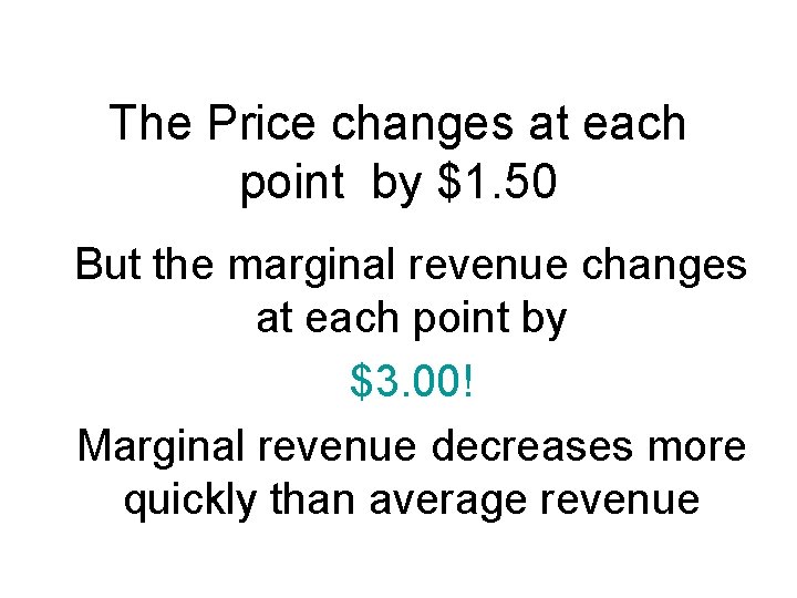
The Price changes at each point by $1. 50 But the marginal revenue changes at each point by $3. 00! Marginal revenue decreases more quickly than average revenue

Will the monopolist ever operate on the inelastic portion of the demand curve? No, the monopolist will never operate on the inelastic portion of the demand curve, because Total Revenue will decline as Price declines beyond the mid-point of the demand curve. Remember the Arc method of elasticity of demand!

Even though marginal revenue is declining, total revenue is increasing, up to the mid-point Beyond the mid-point, marginal revenue is negative, and total revenue begins to decline

Quick review: In the elastic portion of the curve, a change in price results in a bigger percent change in quantity demanded $12 11 10 9 8 7 Costs / Revenue 6 5 D (AR) 4 3 2 1 0 -1 -2 -3 MR 100 200 Quantity 300 400 500 600

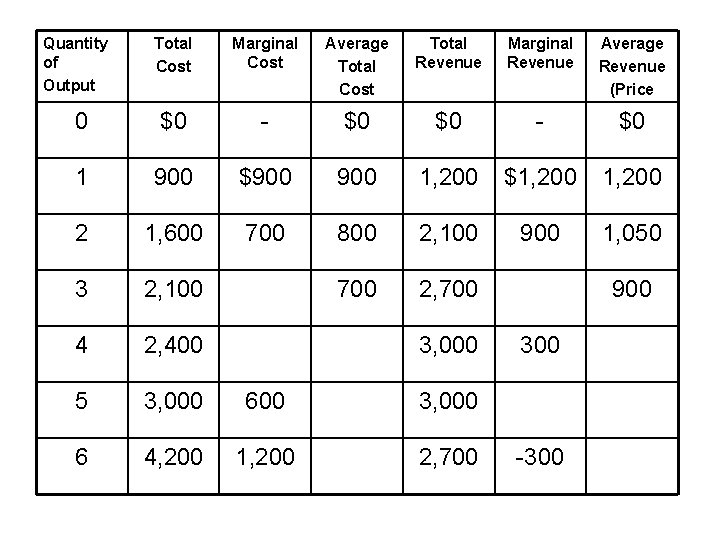
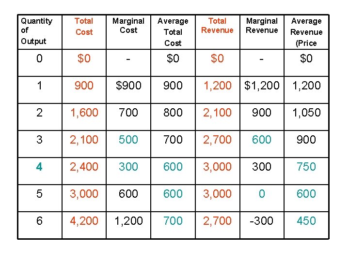
Like the competitive firm, the monopolist will maximize profit at the point of output where marginal cost equals marginal revenue The MC = MR rule

Quantity of Output Total Cost Marginal Cost Average Total Cost Total Revenue Marginal Revenue Average Revenue (Price 0 $0 - $0 1 900 $900 1, 200 $1, 200 2 1, 600 700 800 2, 100 900 1, 050 3 2, 100 700 2, 700 4 2, 400 5 3, 000 600 3, 000 6 4, 200 1, 200 2, 700 3, 000 900 300 -300

Quantity of Output Total Cost Marginal Cost Average Total Cost Total Revenue Marginal Revenue Average Revenue (Price 0 $0 - $0 1 900 $900 1, 200 $1, 200 2 1, 600 700 800 2, 100 900 1, 050 3 2, 100 500 700 2, 700 600 900 4 2, 400 300 600 3, 000 300 750 5 3, 000 600 3, 000 0 600 6 4, 200 1, 200 700 2, 700 -300 450

But, because the marginal revenue curve is below the demand curve, The price at the output level where MC = MR is higher than for a firm in a competitive market, or P > MC not P = MC

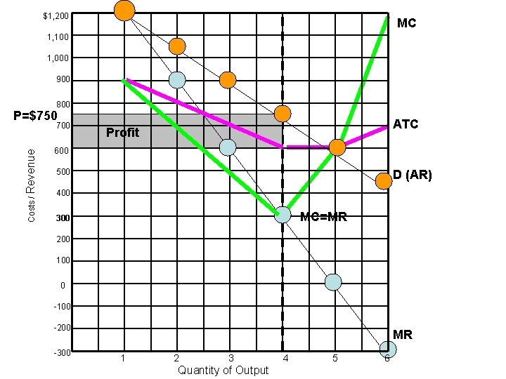
$1, 200 MC 1, 100 1, 000 900 800 P=$750 Costs / Revenue 700 ATC Profit 600 500 D (AR) 400 MC=MR 300 200 100 0 -100 -200 -300 MR 1 2 3 Quantity of Output 4 5 6

• A profit maximizing monopolist would produce an output of 4 units. • At this level of output, MC is $300 per unit and MR is $300 per unit. • At this level of output, ATC is $600 per unit and AR (price) is $750 per unit. • This gives the monopolist an economic profit of $150 per unit for a total economic profit of $600 ($150 x 4)

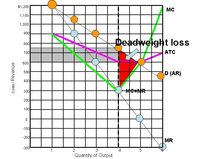
So, The monopolist is inefficient. The marginal cost of the firm is equal to demand (allocative efficiency) at a price of $600 and output of 5 units. But the monopolist charges a higher price and produces less ($750)(4 units) than a firm operating in an efficient competitive market

$1, 200 MC 1, 100 1, 000 900 Deadweight loss 800 ATC Costs / Revenue 700 600 500 D (AR) 400 MC=MR 300 200 100 0 -100 -200 -300 MR 1 2 3 Quantity of Output 4 5 6