Imperfect Competition 1 Pure Monopoly 2 Monopolistic competition

Imperfect Competition 1 -Pure Monopoly 2 -Monopolistic competition 3 -Oligopoly MICROECONOMICS 1 IMPERFECT COMPETITION 1

Pure Monopoly • There is only on seller in the market • Market demand curve is downward sloping • She can either change price or quantity in order to maximize the profit • In order to sell more , she should lower the price • She is facing the market demand individually MICROECONOMICS 1 IMPERFECT COMPETITION 2

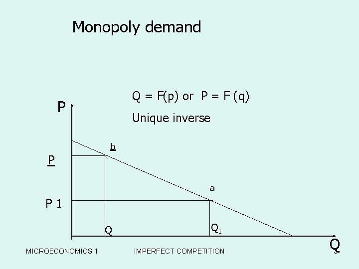
Monopoly demand Q = F(p) or P = F (q) P Unique inverse b P a P 1 Q MICROECONOMICS 1 Q 1 IMPERFECT COMPETITION Q 3

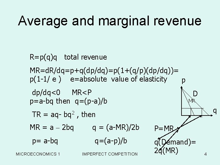
Average and marginal revenue R=p(q)q total revenue MR=d. R/dq=p+q(dp/dq)=p(1+(q/p)(dp/dq))= p(1 -1/ e ) e=absolute value of elasticity p dp/dq<0 MR<P p=a-bq then q=(p-a)/b D MR q TR = aq- bq 2 , then MR = a – 2 bq p= a-bq MICROECONOMICS 1 q = (a-MR)/2 b q=(a-p)/b IMPERFECT COMPETITION P=MR ; q(Demand)= 2 q(MR) 4

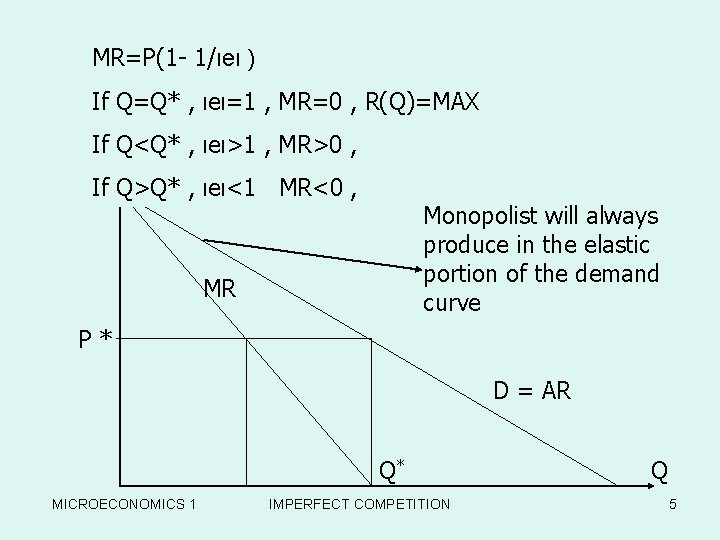
MR=P(1 - 1/ιeι ) If Q=Q* , ιeι=1 , MR=0 , R(Q)=MAX If PQ<Q* , ιeι>1 , MR>0 , If Q>Q* , ιeι<1 MR<0 , Monopolist will always produce in the elastic portion of the demand curve MR P* D = AR Q* MICROECONOMICS 1 IMPERFECT COMPETITION Q 5

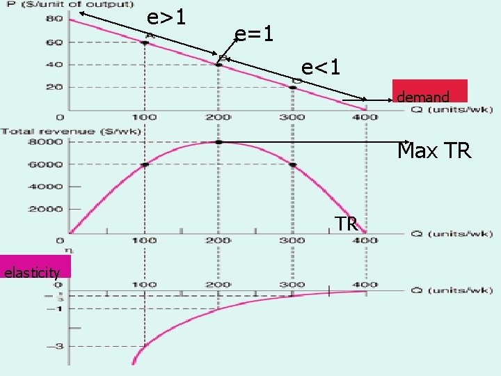
e>1 e=1 Demand, Total Revenue e<1 and Elasticity demand Max TR TR elasticity MICROECONOMICS 1 IMPERFECT COMPETITION 6

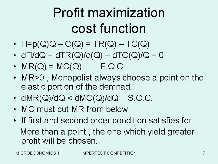
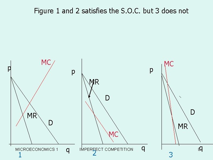
Profit maximization cost function • • П=p(Q)Q – C(Q) = TR(Q) – TC(Q) d. П/d. Q = d. TR(Q)/d(Q) – d. TC(Q)/Q = 0 MR(Q) = MC(Q) F. O. C. MR>0 , Monopolist always choose a point on the elastic portion of the demnad. • d. MR(Q)/d. Q < d. MC(Q)/d. Q S. O. C. • MC must cut MR from below • If first and second order condition satisfies for More than a point , the one which yield greater profit will be chosen. MICROECONOMICS 1 IMPERFECT COMPETITION 7

Figure 1 and 2 satisfies the S. O. C. but 3 does not MC p p p MC MR D D MR MC MICROECONOMICS 1 1 q IMPERFECT COMPETITION 2 q 3 q 8

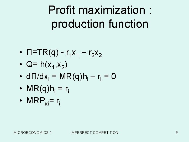
Profit maximization : production function • • • П=TR(q) - r 1 x 1 – r 2 x 2 Q= h(x 1, x 2) d. П/dxi = MR(q)hi – ri = 0 MR(q)hi = ri MRPxi= ri MICROECONOMICS 1 IMPERFECT COMPETITION 9

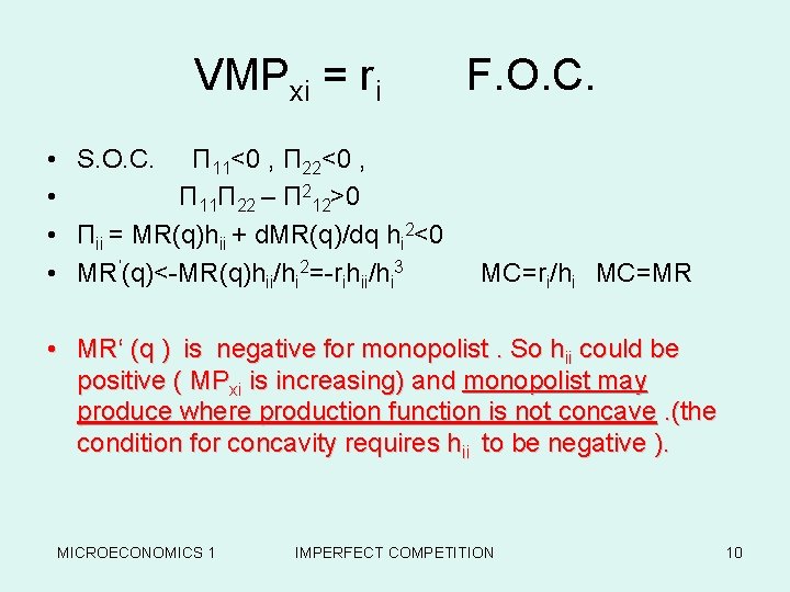
VMPxi = ri • S. O. C. П 11<0 , П 22<0 , • П 11 П 22 – П 212>0 • Пii = MR(q)hii + d. MR(q)/dq hi 2<0 • MR’(q)<-MR(q)hii/hi 2=-rihii/hi 3 F. O. C. MC=ri/hi MC=MR • MR‘ (q ) is negative for monopolist. So hii could be positive ( MPxi is increasing) and monopolist may produce where production function is not concave. (the condition for concavity requires hii to be negative ). MICROECONOMICS 1 IMPERFECT COMPETITION 10

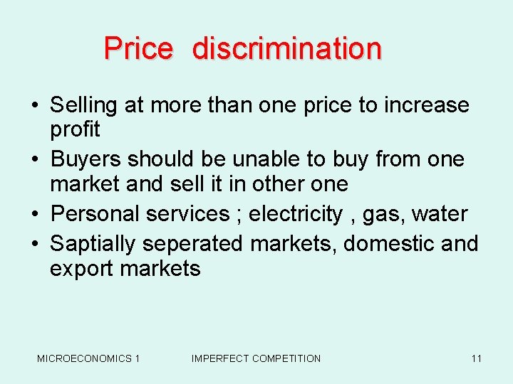
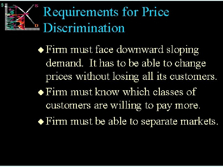
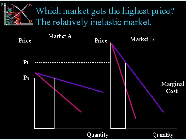
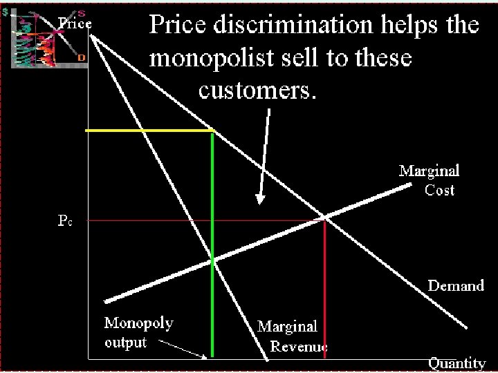
Price discrimination • Selling at more than one price to increase profit • Buyers should be unable to buy from one market and sell it in other one • Personal services ; electricity , gas, water • Saptially seperated markets, domestic and export markets MICROECONOMICS 1 IMPERFECT COMPETITION 11

MICROECONOMICS 1 IMPERFECT COMPETITION 12

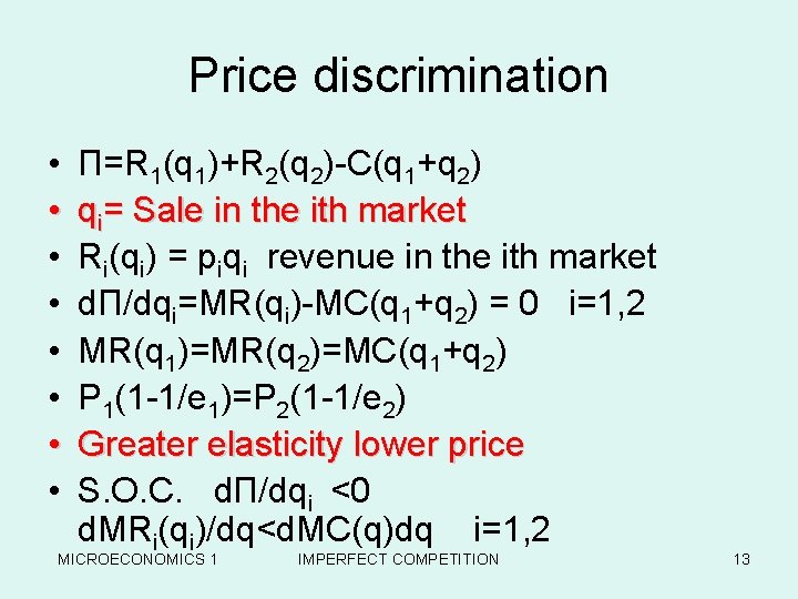
Price discrimination • • П=R 1(q 1)+R 2(q 2)-C(q 1+q 2) qi= Sale in the ith market Ri(qi) = piqi revenue in the ith market d. П/dqi=MR(qi)-MC(q 1+q 2) = 0 i=1, 2 MR(q 1)=MR(q 2)=MC(q 1+q 2) P 1(1 -1/e 1)=P 2(1 -1/e 2) Greater elasticity lower price S. O. C. d. П/dqi <0 d. MRi(qi)/dq<d. MC(q)dq i=1, 2 MICROECONOMICS 1 IMPERFECT COMPETITION 13

MICROECONOMICS 1 IMPERFECT COMPETITION 14

MICROECONOMICS 1 IMPERFECT COMPETITION 15

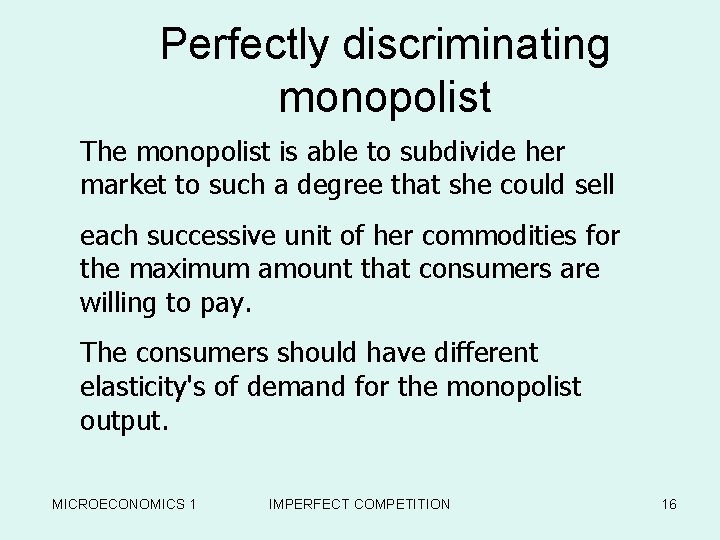
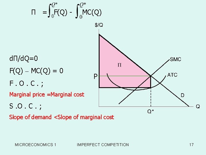
Perfectly discriminating monopolist The monopolist is able to subdivide her market to such a degree that she could sell each successive unit of her commodities for the maximum amount that consumers are willing to pay. The consumers should have different elasticity's of demand for the monopolist output. MICROECONOMICS 1 IMPERFECT COMPETITION 16

П = F(Q) - MC(Q) d. П/d. Q=0 F(Q) – MC(Q) = 0 P F. O. C. ; Marginal price =Marginal cost S. O. C. ; Slope of demand <Slope of marginal cost MICROECONOMICS 1 IMPERFECT COMPETITION 17

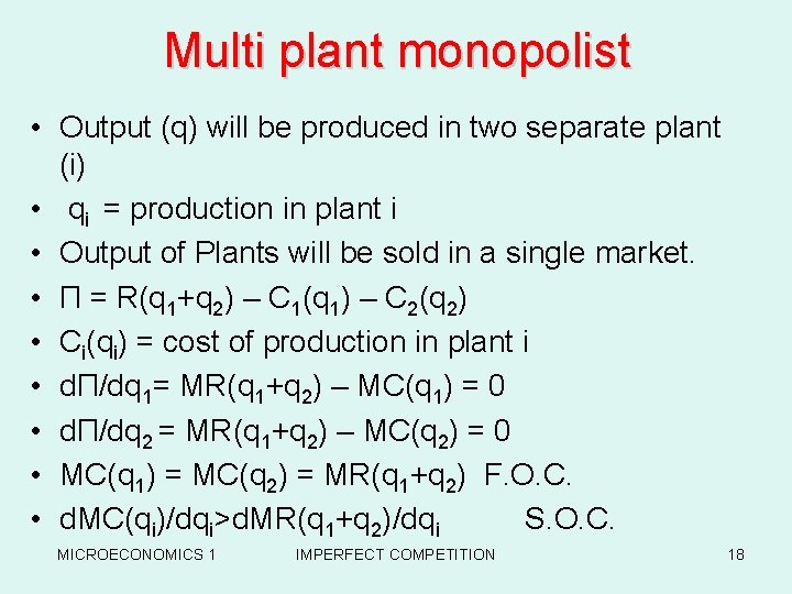
Multi plant monopolist • Output (q) will be produced in two separate plant (i) • qi = production in plant i • Output of Plants will be sold in a single market. • П = R(q 1+q 2) – C 1(q 1) – C 2(q 2) • Ci(qi) = cost of production in plant i • d. П/dq 1= MR(q 1+q 2) – MC(q 1) = 0 • dΠ/dq 2 = MR(q 1+q 2) – MC(q 2) = 0 • MC(q 1) = MC(q 2) = MR(q 1+q 2) F. O. C. • d. MC(qi)/dqi>d. MR(q 1+q 2)/dqi S. O. C. MICROECONOMICS 1 IMPERFECT COMPETITION 18

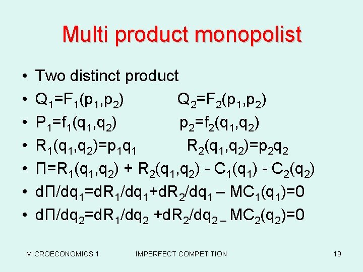
Multi product monopolist • • Two distinct product Q 1=F 1(p 1, p 2) Q 2=F 2(p 1, p 2) P 1=f 1(q 1, q 2) p 2=f 2(q 1, q 2) R 1(q 1, q 2)=p 1 q 1 R 2(q 1, q 2)=p 2 q 2 Π=R 1(q 1, q 2) + R 2(q 1, q 2) - C 1(q 1) - C 2(q 2) dΠ/dq 1=d. R 1/dq 1+d. R 2/dq 1 – MC 1(q 1)=0 dΠ/dq 2=d. R 1/dq 2 +d. R 2/dq 2 – MC 2(q 2)=0 MICROECONOMICS 1 IMPERFECT COMPETITION 19

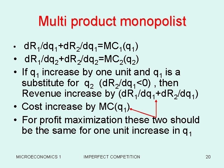
Multi product monopolist • • • d. R 1/dq 1+d. R 2/dq 1=MC 1(q 1) d. R 1/dq 2+d. R 2/dq 2=MC 2(q 2) If q 1 increase by one unit and q 1 is a substitute for q 2 (d. R 2/dq 1<0) , then Revenue increase by (d. R 1/dq 1+d. R 2/dq 1) Cost increase by MC(q 1) For profit maximization these two should be the same for one unit increase in q 1 MICROECONOMICS 1 IMPERFECT COMPETITION 20

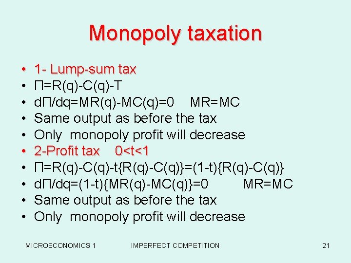
Monopoly taxation • • • 1 - Lump-sum tax Π=R(q)-C(q)-T dΠ/dq=MR(q)-MC(q)=0 MR=MC Same output as before the tax Only monopoly profit will decrease 2 -Profit tax 0<t<1 Π=R(q)-C(q)-t{R(q)-C(q)}=(1 -t){R(q)-C(q)} dΠ/dq=(1 -t){MR(q)-MC(q)}=0 MR=MC Same output as before the tax Only monopoly profit will decrease MICROECONOMICS 1 IMPERFECT COMPETITION 21

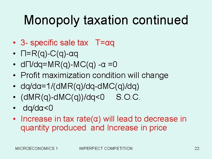
Monopoly taxation continued • • 3 - specific sale tax T=αq Π=R(q)-C(q)-αq dΠ/dq=MR(q)-MC(q) -α =0 Profit maximization condition will change dq/dα=1/(d. MR(q)/dq-d. MC(q)/dq) (d. MR(q)-d. MC(q))/dq<0 S. O. C. dq/dα<0 Increase in tax rate(α) will lead to decrease in quantity produced and Increase in price MICROECONOMICS 1 IMPERFECT COMPETITION 22

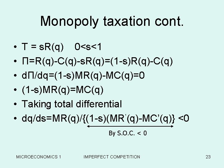
Monopoly taxation cont. • • • T = s. R(q) 0<s<1 Π=R(q)-C(q)-s. R(q)=(1 -s)R(q)-C(q) dΠ/dq=(1 -s)MR(q)-MC(q)=0 (1 -s)MR(q)=MC(q) Taking total differential dq/ds=MR(q)/{(1 -s)(MR’(q)-MC’(q)} <0 By S. O. C. < 0 MICROECONOMICS 1 IMPERFECT COMPETITION 23

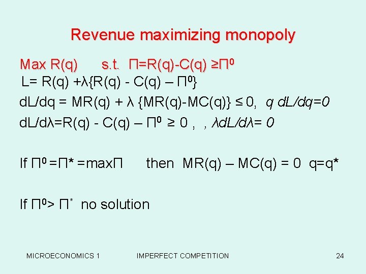
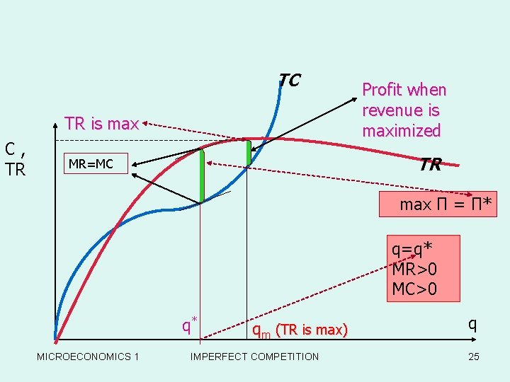
Revenue maximizing monopoly Max R(q) s. t. Π=R(q)-C(q) ≥Π 0 L= R(q) +λ{R(q) - C(q) – Π 0} d. L/dq = MR(q) + λ {MR(q)-MC(q)} ≤ 0, q d. L/dq=0 d. L/dλ=R(q) - C(q) – Π 0 ≥ 0 , , λd. L/dλ= 0 If Π 0 =Π* =maxΠ then MR(q) – MC(q) = 0 q=q* If Π 0> Π* no solution MICROECONOMICS 1 IMPERFECT COMPETITION 24

TC TR is max C, TR Profit when revenue is maximized TR MR=MC max Π = Π* q=q* MR>0 MC>0 q* MICROECONOMICS 1 qm (TR is max) IMPERFECT COMPETITION q 25

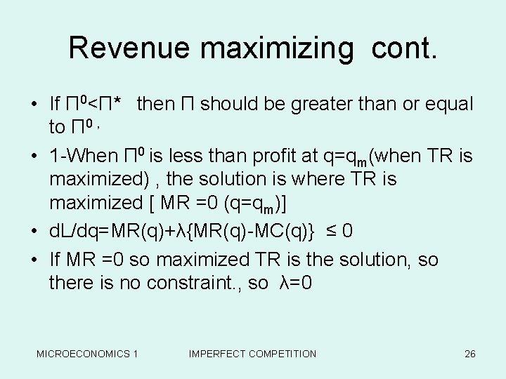
Revenue maximizing cont. • If Π 0<Π* then Π should be greater than or equal to Π 0 , • 1 -When Π 0 is less than profit at q=qm(when TR is maximized) , the solution is where TR is maximized [ MR =0 (q=qm)] • d. L/dq=MR(q)+λ{MR(q)-MC(q)} ≤ 0 • If MR =0 so maximized TR is the solution, so there is no constraint. , so λ=0 MICROECONOMICS 1 IMPERFECT COMPETITION 26

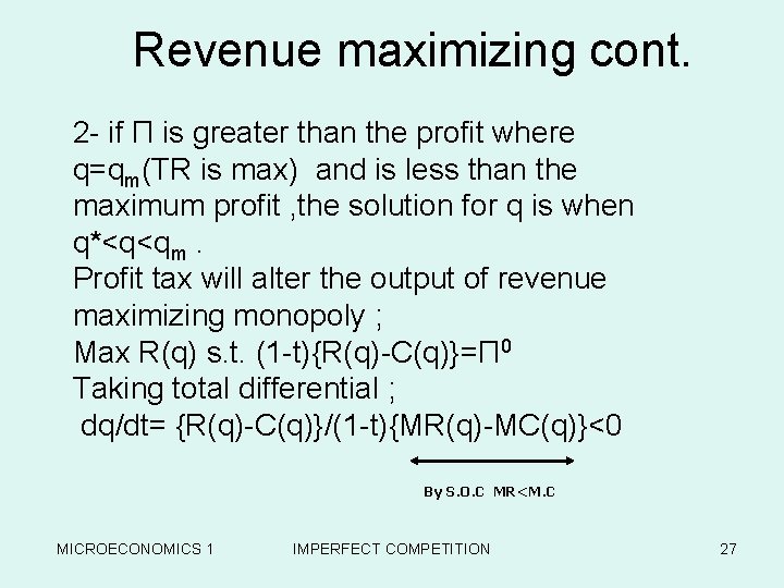
Revenue maximizing cont. 2 - if Π is greater than the profit where q=qm(TR is max) and is less than the maximum profit , the solution for q is when q*<q<qm. Profit tax will alter the output of revenue maximizing monopoly ; Max R(q) s. t. (1 -t){R(q)-C(q)}=Π 0 Taking total differential ; dq/dt= {R(q)-C(q)}/(1 -t){MR(q)-MC(q)}<0 By S. O. C MR<M. C MICROECONOMICS 1 IMPERFECT COMPETITION 27

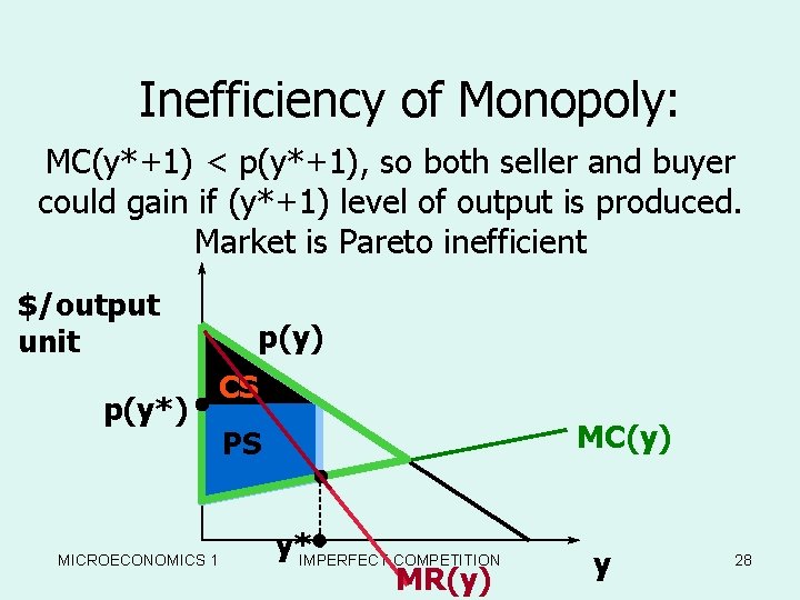
Inefficiency of Monopoly: MC(y*+1) < p(y*+1), so both seller and buyer could gain if (y*+1) level of output is produced. Market is Pareto inefficient $/output unit p(y*) p(y) CS MICROECONOMICS 1 MC(y) PS y*IMPERFECT COMPETITION MR(y) y 28

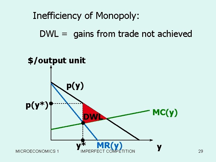
Inefficiency of Monopoly: DWL = gains from trade not achieved $/output unit p(y) p(y*) DWL MICROECONOMICS 1 y* MR(y) IMPERFECT COMPETITION MC(y) y 29

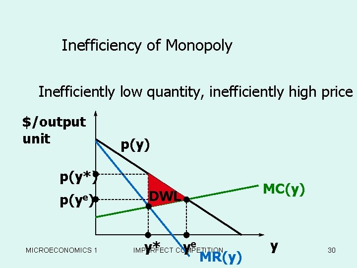
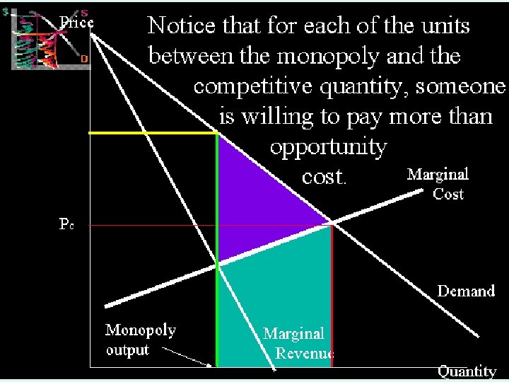
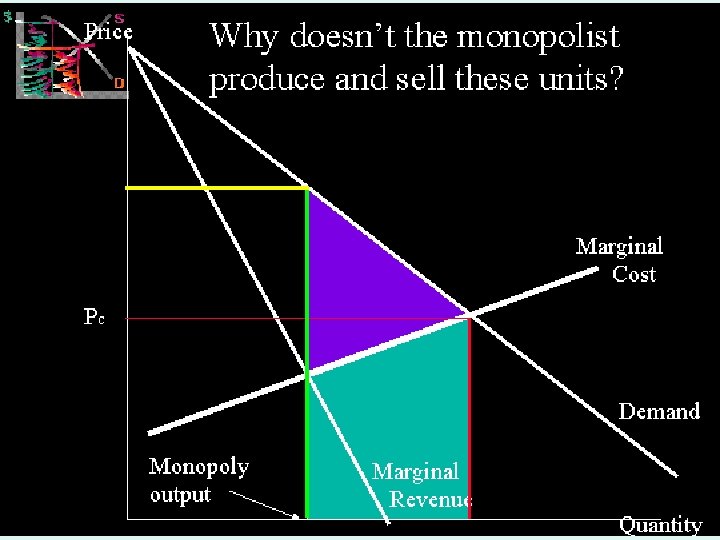
Inefficiency of Monopoly Inefficiently low quantity, inefficiently high price $/output unit p(y) p(y*) p(ye) MICROECONOMICS 1 MC(y) DWL y* ye IMPERFECT COMPETITION MR(y) y 30

MICROECONOMICS 1 IMPERFECT COMPETITION 31

MICROECONOMICS 1 IMPERFECT COMPETITION 32

MICROECONOMICS 1 IMPERFECT COMPETITION 33

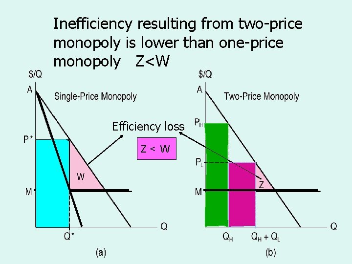
Inefficiency resulting from two-price The Efficiency Losses from monopoly is lower than one-price Single-Price monopoly and Z<WTwo-Price Monopoly Efficiency loss Z< W MICROECONOMICS 1 IMPERFECT COMPETITION 34

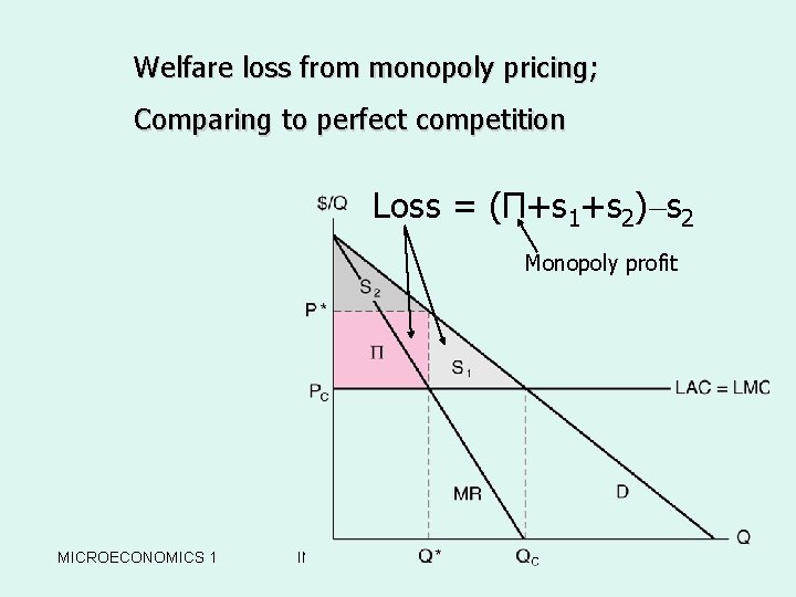
Welfare loss from monopoly pricing; w. The Welfare Loss from Comparing to perfect competition a Single-Price Monopoly Loss = (Π+s 1+s 2)–s 2 Monopoly profit MICROECONOMICS 1 IMPERFECT COMPETITION 35

MICROECONOMICS 1 IMPERFECT COMPETITION 36

MICROECONOMICS 1 IMPERFECT COMPETITION 37

MICROECONOMICS 1 IMPERFECT COMPETITION 38

MICROECONOMICS 1 IMPERFECT COMPETITION 39

MICROECONOMICS 1 IMPERFECT COMPETITION 40

MICROECONOMICS 1 IMPERFECT COMPETITION 41

MICROECONOMICS 1 IMPERFECT COMPETITION 42

MICROECONOMICS 1 IMPERFECT COMPETITION 43

MICROECONOMICS 1 IMPERFECT COMPETITION 44

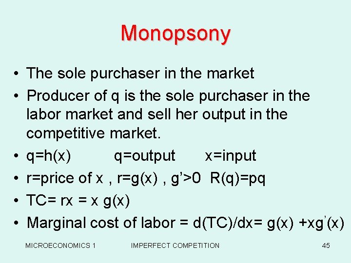
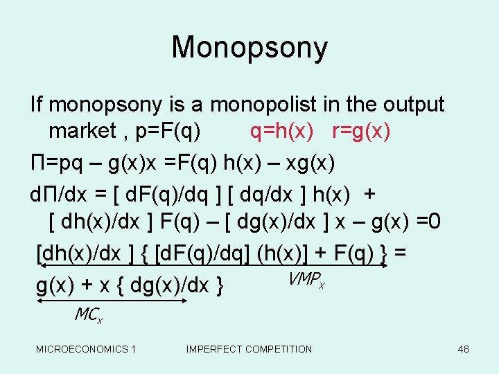
Monopsony • The sole purchaser in the market • Producer of q is the sole purchaser in the labor market and sell her output in the competitive market. • q=h(x) q=output x=input • r=price of x , r=g(x) , g’>0 R(q)=pq • TC= rx = x g(x) • Marginal cost of labor = d(TC)/dx= g(x) +xg’(x) MICROECONOMICS 1 IMPERFECT COMPETITION 45

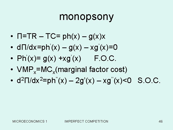
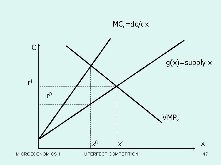
monopsony • • • Π=TR – TC= ph(x) – g(x)x dΠ/dx=ph’(x) – g(x) – xg’(x)=0 Ph’(x)= g(x) +xg’(x) F. O. C. VMPx=MCx(marginal factor cost) d 2Π/dx 2=ph’’(x) – 2 g’(x) – xg’’(x)<0 S. O. C. MICROECONOMICS 1 IMPERFECT COMPETITION 46

MCx=dc/dx C g(x)=supply x r 1 r 0 VMPx x 0 MICROECONOMICS 1 x 1 IMPERFECT COMPETITION x 47

Monopsony If monopsony is a monopolist in the output market , p=F(q) q=h(x) r=g(x) Π=pq – g(x)x =F(q) h(x) – xg(x) dΠ/dx = [ d. F(q)/dq ] [ dq/dx ] h(x) + [ dh(x)/dx ] F(q) – [ dg(x)/dx ] x – g(x) =0 [dh(x)/dx ] { [d. F(q)/dq] (h(x)] + F(q) } = VMPx g(x) + x { dg(x)/dx } MCx MICROECONOMICS 1 IMPERFECT COMPETITION 48

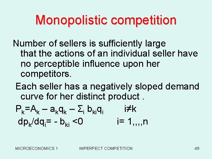
Monopolistic competition Number of sellers is sufficiently large that the actions of an individual seller have no perceptible influence upon her competitors. Each seller has a negatively sloped demand curve for her distinct product. Pk=Ak – akqk – Σi bkiqi i≠k dpk/dqi= - bki <0 i= 1, , n MICROECONOMICS 1 IMPERFECT COMPETITION 49

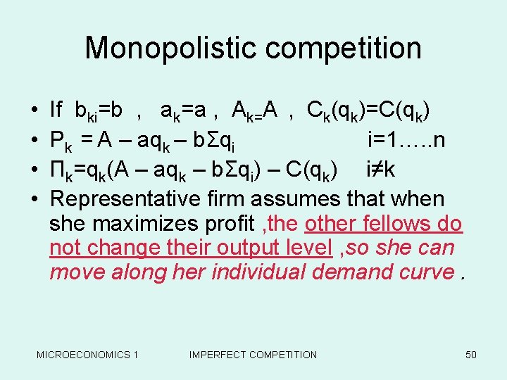
Monopolistic competition • • If bki=b , ak=a , Ak=A , Ck(qk)=C(qk) Pk = A – aqk – bΣqi i=1…. . n Πk=qk(A – aqk – bΣqi) – C(qk) i≠k Representative firm assumes that when she maximizes profit , the other fellows do not change their output level , so she can move along her individual demand curve. MICROECONOMICS 1 IMPERFECT COMPETITION 50

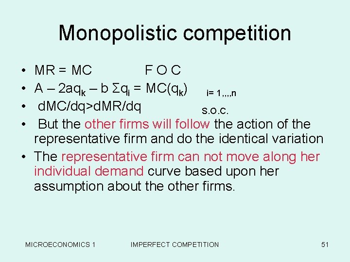
Monopolistic competition • • MR = MC FOC A – 2 aqk – b Σqi = MC(qk) i= 1, , n d. MC/dq>d. MR/dq S. O. C. But the other firms will follow the action of the representative firm and do the identical variation • The representative firm can not move along her individual demand curve based upon her assumption about the other firms. MICROECONOMICS 1 IMPERFECT COMPETITION 51

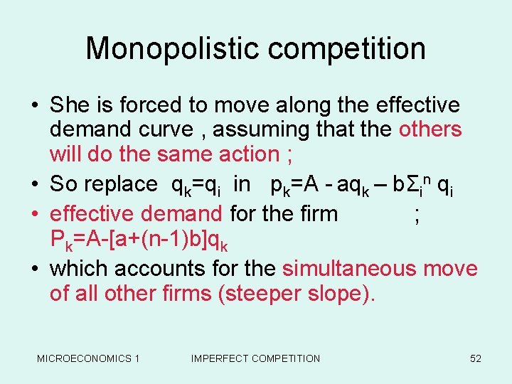
Monopolistic competition • She is forced to move along the effective demand curve , assuming that the others will do the same action ; • So replace qk=qi in pk=A - aqk – bΣin qi • effective demand for the firm ; Pk=A-[a+(n-1)b]qk • which accounts for the simultaneous move of all other firms (steeper slope). MICROECONOMICS 1 IMPERFECT COMPETITION 52

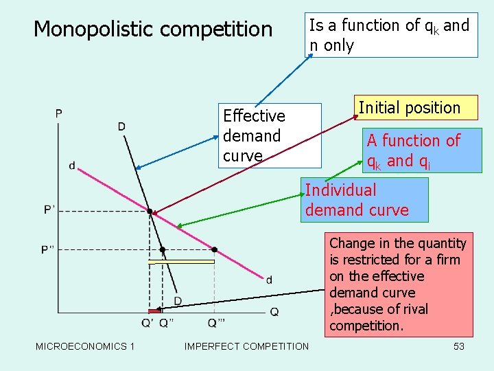
Monopolistic competition Is a function of qk and n only Competitor’s The Monopolistic Competitor’s Two Demand Curves Initial position Effective demand curve A function of qk and qi Individual demand curve Change in the quantity is restricted for a firm on the effective demand curve , because of rival competition. MICROECONOMICS 1 IMPERFECT COMPETITION 53

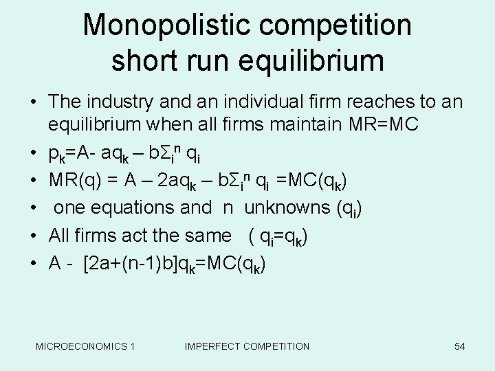
Monopolistic competition short run equilibrium • The industry and an individual firm reaches to an equilibrium when all firms maintain MR=MC • pk=A- aqk – bΣin qi • MR(q) = A – 2 aqk – bΣin qi =MC(qk) • one equations and n unknowns (qi) • All firms act the same ( qi=qk) • A - [2 a+(n-1)b]qk=MC(qk) MICROECONOMICS 1 IMPERFECT COMPETITION 54

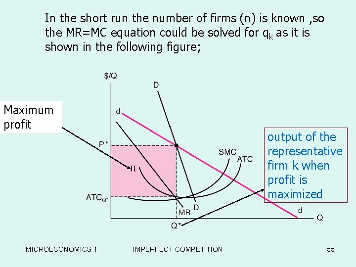
In the short run the number of firms (n) is known , so the MR=MC equation could be solved for qk as it is shown. Equilibrium in the following figure; -Run for the Maximum profit MICROECONOMICS 1 output of the representative firm k when profit is maximized IMPERFECT COMPETITION 55

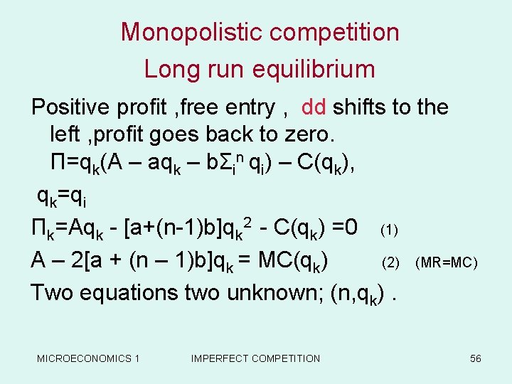
Monopolistic competition Long run equilibrium Positive profit , free entry , dd shifts to the left , profit goes back to zero. Π=qk(A – aqk – bΣin qi) – C(qk), qk=qi Πk=Aqk - [a+(n-1)b]qk 2 - C(qk) =0 (1) A – 2[a + (n – 1)b]qk = MC(qk) (2) (MR=MC) Two equations two unknown; (n, qk). MICROECONOMICS 1 IMPERFECT COMPETITION 56

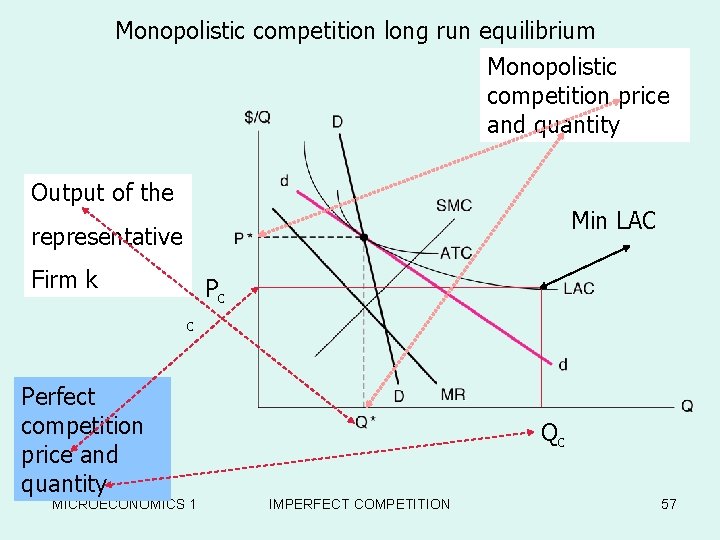
Monopolistic competition long run equilibrium Monopolistic Long-Run Equilibrium in the competition price Chamberlain Model and quantity Output of the Min LAC representative Firm k Pc c Perfect competition price and quantity MICROECONOMICS 1 Qc IMPERFECT COMPETITION 57

Oligopoly • The result of any move on the part of a oligopolies depend upon the reactions of his rivals. • General price-quantity relationship can not be defined, because he can not control the output of other firms. It depends to the assumption which we make about the behavior of his rivals. MICROECONOMICS 1 IMPERFECT COMPETITION 58

Oligopoly • If dΠi/dqj is negligible we will have perfect competition or monopolistic competition. • If dΠi/dqj is noticeable we will have duopolistic or oligopolist • Different assumptions about the behavior of the rivals leads to different models of oligopoly. these assumptions may be as follows ; MICROECONOMICS 1 IMPERFECT COMPETITION 59

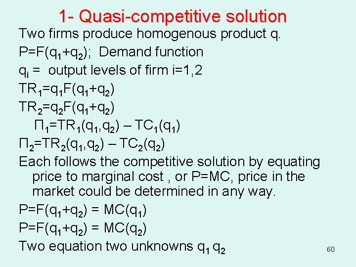
1 - Quasi-competitive solution Two firms produce homogenous product q. P=F(q 1+q 2); Demand function qi = output levels of firm i=1, 2 TR 1=q 1 F(q 1+q 2) TR 2=q 2 F(q 1+q 2) Π 1=TR 1(q 1, q 2) – TC 1(q 1) Π 2=TR 2(q 1, q 2) – TC 2(q 2) Each follows the competitive solution by equating price to marginal cost , or P=MC, price in the market could be determined in any way. P=F(q 1+q 2) = MC(q 1) P=F(q 1+q 2) = MC(q 2) Two equation two unknowns q 1 q 2 60

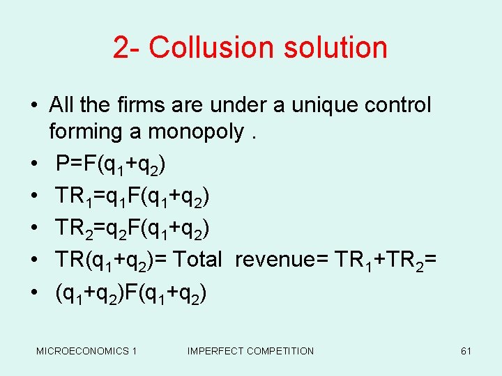
2 - Collusion solution • All the firms are under a unique control forming a monopoly. • P=F(q 1+q 2) • TR 1=q 1 F(q 1+q 2) • TR 2=q 2 F(q 1+q 2) • TR(q 1+q 2)= Total revenue= TR 1+TR 2= • (q 1+q 2)F(q 1+q 2) MICROECONOMICS 1 IMPERFECT COMPETITION 61

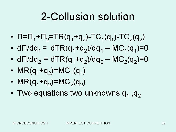
2 -Collusion solution • • • Π=Π 1+Π 2=TR(q 1+q 2)-TC 1(q 1)-TC 2(q 2) dΠ/dq 1 = d. TR(q 1+q 2)/dq 1 – MC 1(q 1)=0 dΠ/dq 2 = d. TR(q 1+q 2)/dq 2 – MC 2(q 2)=0 MR(q 1+q 2)=MC 1(q 1) MR(q 1+q 2)=MC 2(q 2) Two equations two unknowns q 1 , q 2 MICROECONOMICS 1 IMPERFECT COMPETITION 62

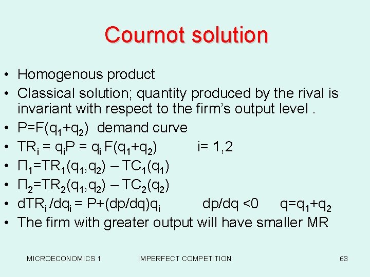
Cournot solution • Homogenous product • Classical solution; quantity produced by the rival is invariant with respect to the firm’s output level. • P=F(q 1+q 2) demand curve • TRi = qi. P = qi F(q 1+q 2) i= 1, 2 • Π 1=TR 1(q 1, q 2) – TC 1(q 1) • Π 2=TR 2(q 1, q 2) – TC 2(q 2) • d. TRi /dqi = P+(dp/dq)qi dp/dq <0 q=q 1+q 2 • The firm with greater output will have smaller MR MICROECONOMICS 1 IMPERFECT COMPETITION 63

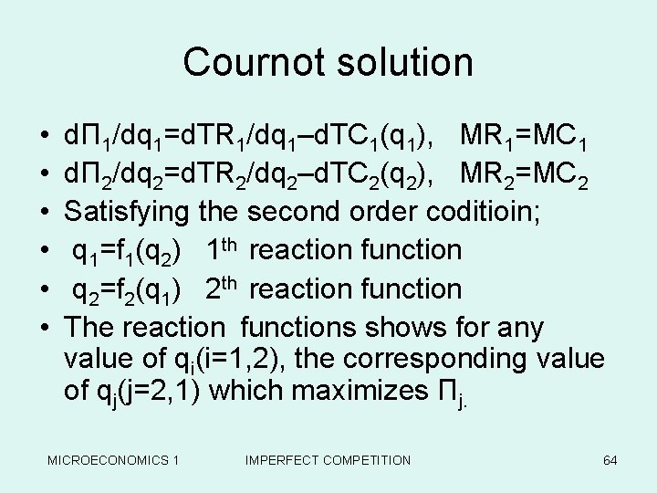
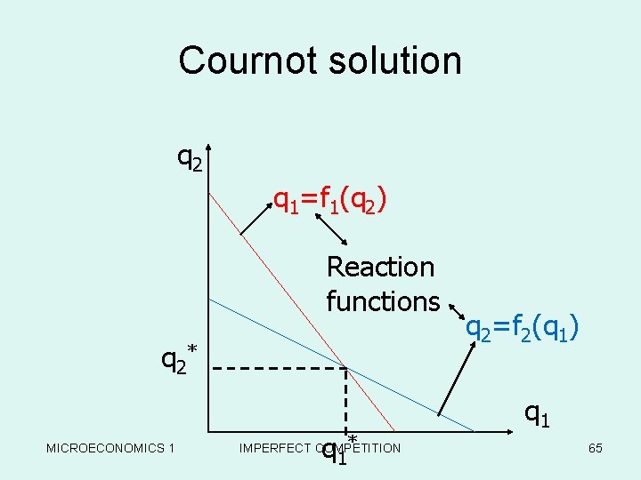
Cournot solution • • • dΠ 1/dq 1=d. TR 1/dq 1–d. TC 1(q 1), MR 1=MC 1 dΠ 2/dq 2=d. TR 2/dq 2–d. TC 2(q 2), MR 2=MC 2 Satisfying the second order coditioin; q 1=f 1(q 2) 1 th reaction function q 2=f 2(q 1) 2 th reaction function The reaction functions shows for any value of qi(i=1, 2), the corresponding value of qj(j=2, 1) which maximizes Πj. MICROECONOMICS 1 IMPERFECT COMPETITION 64

Cournot solution q 2 q 1=f 1(q 2) Reaction functions q 2* MICROECONOMICS 1 q 1 * IMPERFECT COMPETITION q 2=f 2(q 1) q 1 65

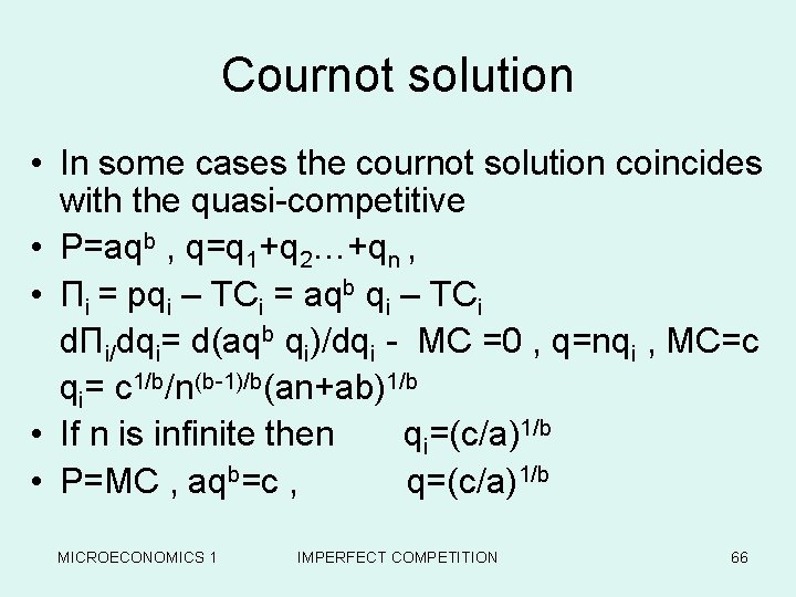
Cournot solution • In some cases the cournot solution coincides with the quasi-competitive • P=aqb , q=q 1+q 2…+qn , • Πi = pqi – TCi = aqb qi – TCi dΠi/dqi= d(aqb qi)/dqi - MC =0 , q=nqi , MC=c qi= c 1/b/n(b-1)/b(an+ab)1/b • If n is infinite then qi=(c/a)1/b • P=MC , aqb=c , q=(c/a)1/b MICROECONOMICS 1 IMPERFECT COMPETITION 66

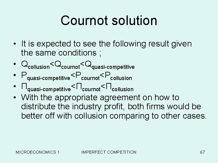
Cournot solution • It is expected to see the following result given the same conditions ; • Qcollusion<Qcournot<Qquasi-competitive • Pquasi-competitive<Pcournot<Pcollusion • Πquasi-competitive<Πcournot<Πcollusion • With the appropriate agreement on how to distribute the industry profit, both firms would be better off with collusion comparing to other cases. MICROECONOMICS 1 IMPERFECT COMPETITION 67

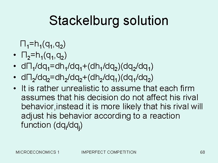
Stackelburg solution • • Π 1=h 1(q 1, q 2) Π 2=h 1(q 1, q 2) dΠ 1/dq 1=dh 1/dq 1+(dh 1/dq 2)(dq 2/dq 1) dΠ 2/dq 2=dh 2/dq 2+(dh 2/dq 1)(dq 1/dq 2) It is rather unrealistic to assume that each firm assumes that his decision do not affect his rival behavior, instead it is more likely that his rival will adjust his behavior according to a reaction function (dqi/dqj) MICROECONOMICS 1 IMPERFECT COMPETITION 68

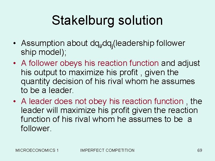
Stakelburg solution • Assumption about dqi/dqj(leadership follower ship model); • A follower obeys his reaction function and adjust his output to maximize his profit , given the quantity decision of his rival whom he assumes to be a leader. • A leader does not obey his reaction function , the leader will maximize his profit given the reaction function of his rival whom he assumes to be a follower. MICROECONOMICS 1 IMPERFECT COMPETITION 69

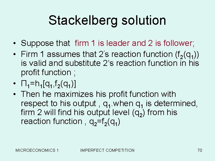
Stackelberg solution • Suppose that firm 1 is leader and 2 is follower; • Firm 1 assumes that 2’s reaction function (f 2(q 1)) is valid and substitute 2’s reaction function in his profit function ; • Π 1=h 1[q 1, f 2(q 1)] • Then he maximizes his profit function with respect to his output , q 1. when q 1 is determined, firm 2 will find his output level (q 2) from his reaction function , q 2=f 2(q 1) MICROECONOMICS 1 IMPERFECT COMPETITION 70

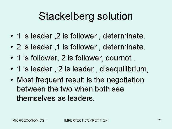
Stackelberg solution • • • 1 is leader , 2 is follower , determinate. 2 is leader , 1 is follower , determinate. 1 is follower, 2 is follower, cournot. 1 is leader , 2 is leader , disequilibrium, Most frequent result is the negotiation between the two when both see themselves as leaders. MICROECONOMICS 1 IMPERFECT COMPETITION 71

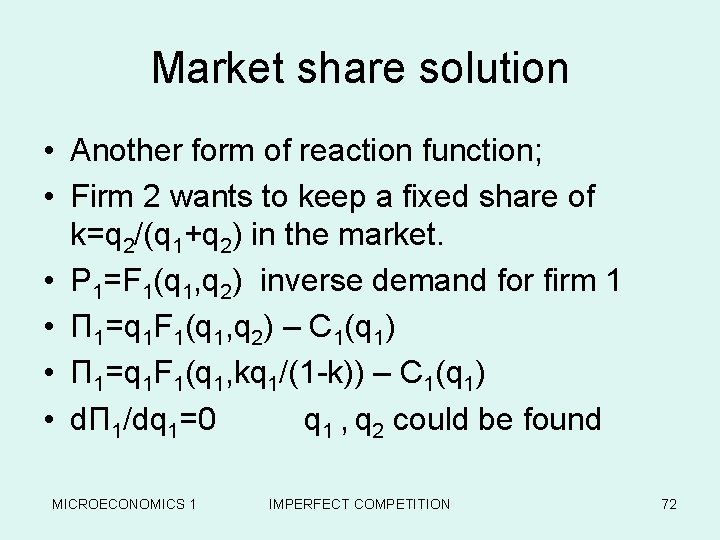
Market share solution • Another form of reaction function; • Firm 2 wants to keep a fixed share of k=q 2/(q 1+q 2) in the market. • P 1=F 1(q 1, q 2) inverse demand for firm 1 • Π 1=q 1 F 1(q 1, q 2) – C 1(q 1) • Π 1=q 1 F 1(q 1, kq 1/(1 -k)) – C 1(q 1) • dΠ 1/dq 1=0 q 1 , q 2 could be found MICROECONOMICS 1 IMPERFECT COMPETITION 72

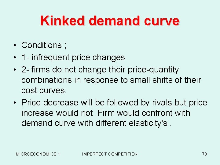
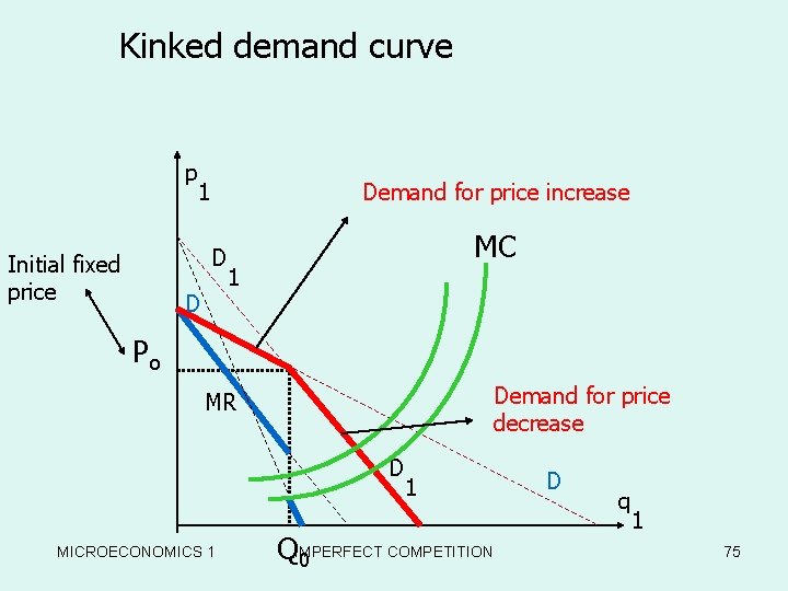
Kinked demand curve • Conditions ; • 1 - infrequent price changes • 2 - firms do not change their price-quantity combinations in response to small shifts of their cost curves. • Price decrease will be followed by rivals but price increase would not. Firm would confront with demand curve with different elasticity's. MICROECONOMICS 1 IMPERFECT COMPETITION 73

Kinked demand curve • So marginal revenue curve will be broken. • Variation of marginal cost in the broken area of marginal revenue does not change the price. MICROECONOMICS 1 IMPERFECT COMPETITION 74

Kinked demand curve p 1 Demand for price increase D Initial fixed price D MC 1 Po Demand for price decrease MR D MICROECONOMICS 1 1 COMPETITION QIMPERFECT 0 D q 1 75

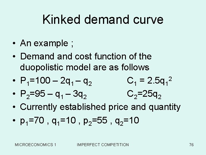
Kinked demand curve • An example ; • Demand cost function of the duopolistic model are as follows • P 1=100 – 2 q 1 – q 2 C 1 = 2. 5 q 12 • P 2=95 – q 1 – 3 q 2 C 2=25 q 2 • Currently established price and quantity • p 1=70 , q 1=10 , p 2=55 , q 2=10 MICROECONOMICS 1 IMPERFECT COMPETITION 76

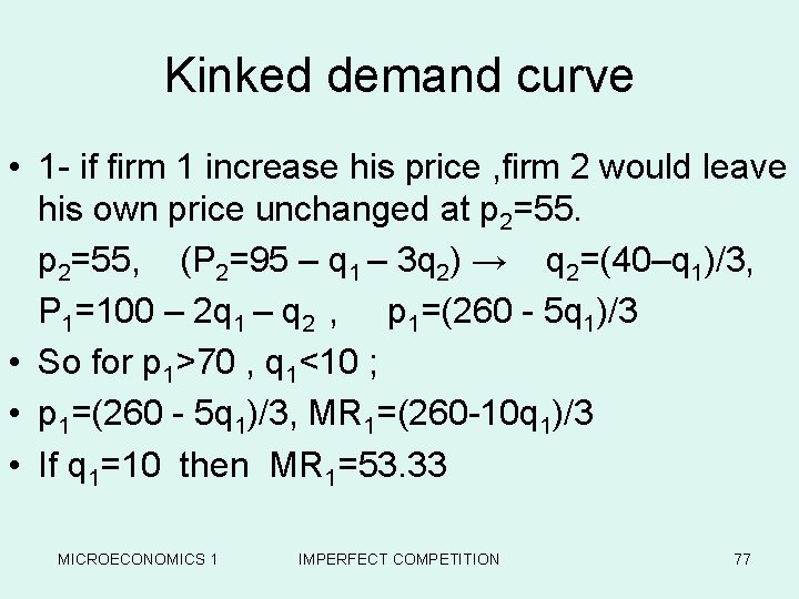
Kinked demand curve • 1 - if firm 1 increase his price , firm 2 would leave his own price unchanged at p 2=55, (P 2=95 – q 1 – 3 q 2) → q 2=(40–q 1)/3, P 1=100 – 2 q 1 – q 2 , p 1=(260 - 5 q 1)/3 • So for p 1>70 , q 1<10 ; • p 1=(260 - 5 q 1)/3, MR 1=(260 -10 q 1)/3 • If q 1=10 then MR 1=53. 33 MICROECONOMICS 1 IMPERFECT COMPETITION 77

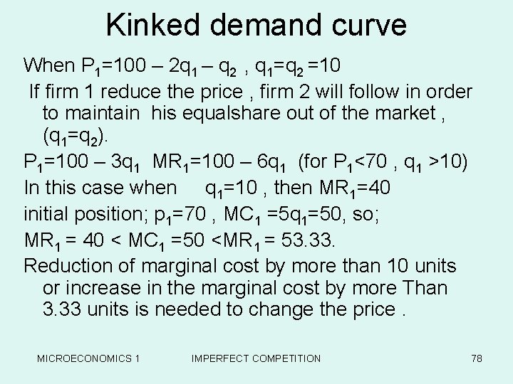
Kinked demand curve When P 1=100 – 2 q 1 – q 2 , q 1=q 2 =10 If firm 1 reduce the price , firm 2 will follow in order to maintain his equalshare out of the market , (q 1=q 2). P 1=100 – 3 q 1 MR 1=100 – 6 q 1 (for P 1<70 , q 1 >10) In this case when q 1=10 , then MR 1=40 initial position; p 1=70 , MC 1 =5 q 1=50, so; MR 1 = 40 < MC 1 =50 <MR 1 = 53. 33. Reduction of marginal cost by more than 10 units or increase in the marginal cost by more Than 3. 33 units is needed to change the price. MICROECONOMICS 1 IMPERFECT COMPETITION 78

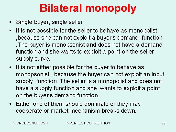
Bilateral monopoly • Single buyer, single seller • It is not possible for the seller to behave as monopolist , because she can not exploit a buyer’s demand function. The buyer is monopsonist and does not have a demand function and she wants to exploit a point on the seller supply curve. • It is not either possible for the buyer to behave as monopsonist , because the buyer can not exploit an input supply function. The seller is a monopolist and does not have a supply function and she wants to exploit a point on the buyer’s demand function. • Either one of them should dominate or they may cooperate or market mechanism breaks down. MICROECONOMICS 1 IMPERFECT COMPETITION 79

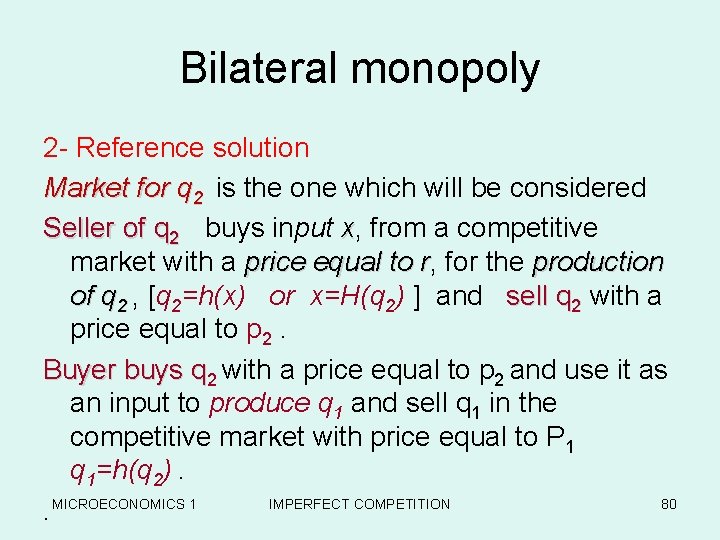
Bilateral monopoly 2 - Reference solution Market for q 2 is the one which will be considered Seller of q 2 buys input x, from a competitive market with a price equal to r, r for the production of q 2 , [q 2=h(x) or x=H(q 2) ] and sell q 2 with a price equal to p 2. Buyer buys q 2 with a price equal to p 2 and use it as an input to produce q 1 and sell q 1 in the competitive market with price equal to P 1 q 1=h(q 2). IMPERFECT COMPETITION 80. MICROECONOMICS 1

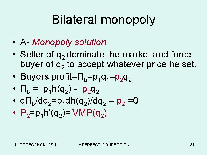
Bilateral monopoly • A- Monopoly solution • Seller of q 2 dominate the market and force buyer of q 2 to accept whatever price he set. • Buyers profit=Πb=p 1 q 1–p 2 q 2 • Πb = p 1 h(q 2) - p 2 q 2 • dΠb/dq 2=p 1 dh(q 2)/dq 2 – p 2 =0 • P 2=p 1 h’(q 2)= VMP(q 2) MICROECONOMICS 1 IMPERFECT COMPETITION 81

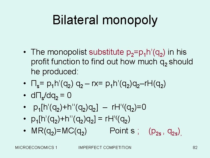
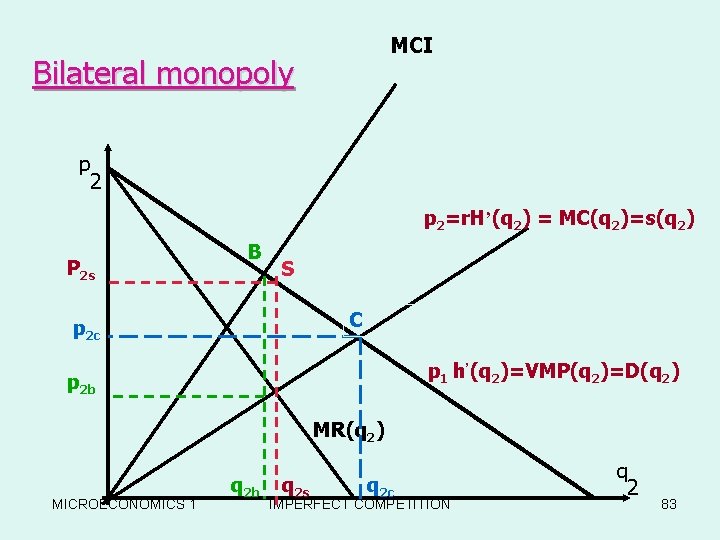
Bilateral monopoly • The monopolist substitute p 2=p 1 h’(q 2) in his profit function to find out how much q 2 should he produced: • Πs= p 1 h’(q 2) q 2 – rx= p 1 h’(q 2)q 2–r. H(q 2) • dΠs/dq 2 = 0 • p 1[h’(q 2)+h’’(q 2)q 2] – r. H’((q 2)=0 • p 1[h’(q 2)+h’’(q 2)q 2] = r. H’((q 2) • MR(q 2)=MC(q 2) Point s ; (p 2 s , q 2 s), MICROECONOMICS 1 IMPERFECT COMPETITION 82

MCI Bilateral monopoly p 2=r. H’(q 2) = MC(q 2)=s(q 2) P 2 s B S C p 2 c p 1 h’(q 2)=VMP(q 2)=D(q 2) p 2 b MR(q 2) MICROECONOMICS 1 q 2 b q 2 s q 2 c IMPERFECT COMPETITION q 2 83

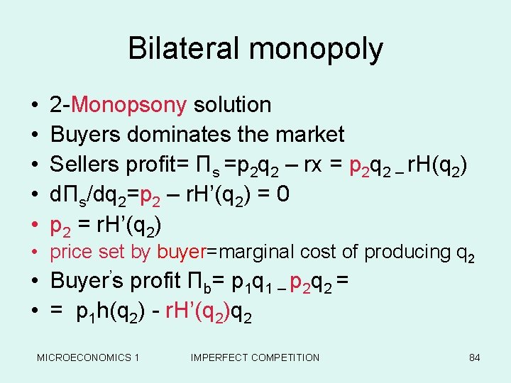
Bilateral monopoly • • • 2 -Monopsony solution Buyers dominates the market Sellers profit= Πs =p 2 q 2 – rx = p 2 q 2 – r. H(q 2) dΠs/dq 2=p 2 – r. H’(q 2) = 0 p 2 = r. H’(q 2) • price set by buyer=marginal cost of producing q 2 • Buyer’s profit Πb= p 1 q 1 – p 2 q 2 = • = p 1 h(q 2) - r. H’(q 2)q 2 MICROECONOMICS 1 IMPERFECT COMPETITION 84

Bilateral monopoly dΠb / dq 2=p 1 h’(q 2)-r[H’(q 2)+H’’(q 2)q 2]=0 p 1 h’(q 2) = r[H’(q 2)+H’’(q 2)q 2] VMP(q 2 in producing q 1)=MC of buying q 2 for buyer Point B in the figure, q 2=q 2 b, p 2=p 2 b 3 - Seller and buyer are both price taker ( quasi competitive solution ) Supply and demand function are effective ; point c , p 2=p 2 c , q 2=q 2 c P 1 h’(q 2 c)=r. H’(q 2 c) VMP(q 2 in producing q 1)=MC(q 2) for seller MICROECONOMICS 1 IMPERFECT COMPETITION 85

Bilateral monopoly • As a rule ; q 2 c>q 2 b , q 2 c>q 2 s , but • Relation between q 2 b and q 2 s is not kwon. It depends to the position (elasticity) of supply and demand curves. • In general we expect to have the following results given the same conditions ; • P 2 b<P 2 c<P 2 s • Πss> Πsc> Πsb seller’ s profit in three cases • Πbs< Πbc< Πbb buyer’s profit in three cases MICROECONOMICS 1 IMPERFECT COMPETITION 86

Bilateral monopoly • 4 - Collusion and bargaining • This happens to reach to an agreement on unique price and quantity. This includes two process; • 1 - determining (q) such that their joint profit is maximized. • 2 - determining (P) in order to distribute the profit MICROECONOMICS 1 IMPERFECT COMPETITION 87

Bilateral monopoly • • Π=Πb+Πs=[p 1 h(q 2)–p 2 q 2]+[p 2 q 2 -r. H(q 2)] dΠ/dq 2=p 1 h’(q 2) – r. H’(q 2)=0 p 1 h’(q 2)=r. H’(q 2) (q 2=q 2 c) VMP(q 2 in producing q 1) = Marginal cost of q 2 for seller • Quasi-competitive price does not necessarily follow from a collusive solution. • The seller wants to put the price as high as possible. • Buyer wants to put the price as low as possible. MICROECONOMICS 1 IMPERFECT COMPETITION 88

Bilateral monopoly • Different solutions can be found for price (p 2); • 1 - P** <P 2<P* • Price that force the buyer’s profit to zero = p*= [p 1 h(q 2 c)]/q 2 c • Price that force the seller’s profit to zero = p**= [r. H(q 2 c)]/q 2 c • 2 - Buyer can do no worse than monopoly situation and seller can do no worse than monopsony solution. MICROECONOMICS 1 IMPERFECT COMPETITION 89

Bilateral monopoly • Buyer’s profit in monopoly situation= • P 1 h(q 2 c) – p 2 q 2 c = Πbs • P’ 2=[p 1 h(q 2 c) – Πbs] /q 2 c • • • Seller’s profit in monopsony situation= p 2 q 2 c – r. H(q 2 c) = Πsb P’’ 2=[r. H(q 2 c) + Πsb]/q 2 c P’’ 2<P’ 2 In each case the determination of p 2 depends upon the relative power of the bargaining process. • MICROECONOMICS 1 IMPERFECT COMPETITION 90

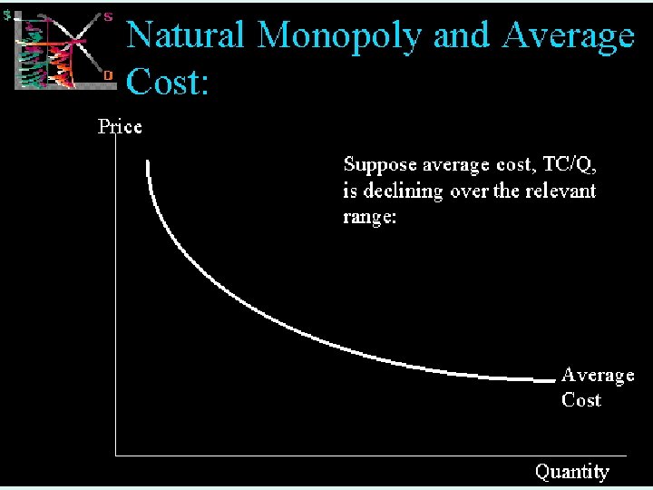
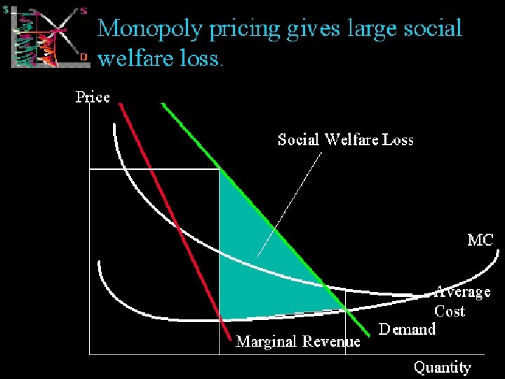
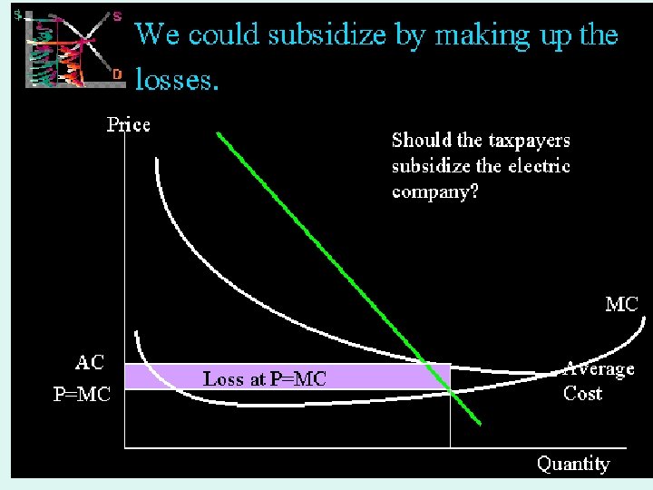
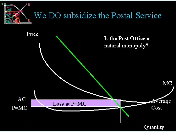
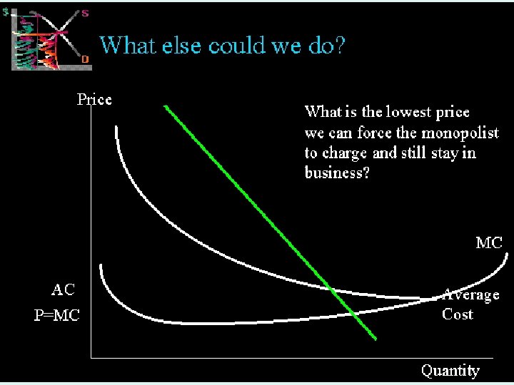
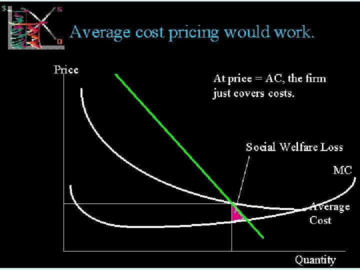
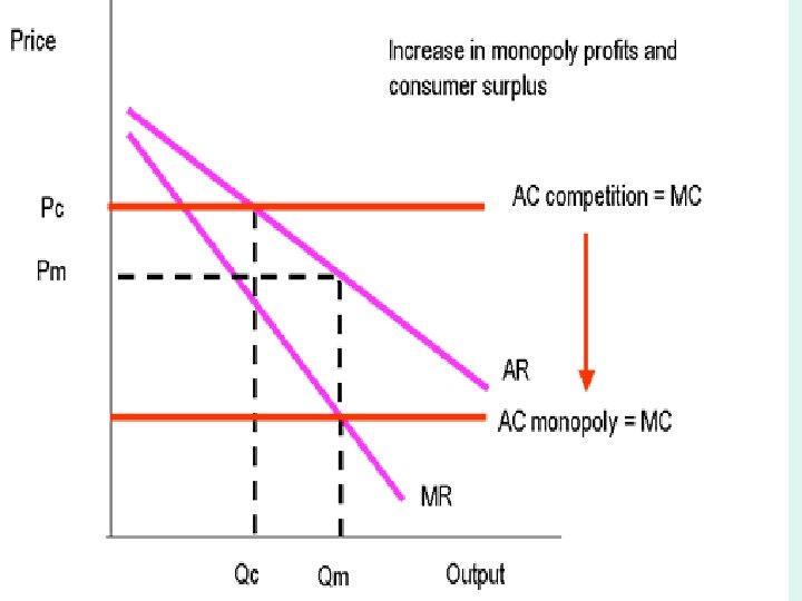
• CAN MONOPOLY BE DEFENDED? • Monopoly and Economies of Scale • Because monopoly producers are often supplying goods and services on a very large scale they may be better placed to take advantage of economies of scale - leading to a fall in the average total costs of production. These reductions in costs will lead to an increase in monopoly profits but some of the gains in productive efficiency might be passed onto consumers in the form of lower prices. The effect of economies of scale is shown in the diagram. • As shown in the following figure economies of scale provide potential gains in economic welfare for both producers and consumers. MICROECONOMICS 1 IMPERFECT COMPETITION 91 • .

MICROECONOMICS 1 IMPERFECT COMPETITION 92

• • Monopoly and Innovation (Research and Development) How are the supernormal profits of monopoly used? Is consumer surplus of equal value to producer surplus? Are large-scale firms required to create a comparative advantage in global markets? Some economists argue that large-scale firms are required to be competitive in international markets An important issue is what happens to the monopoly profits both in the short run and the long run. Undoubtedly some of the profits will be distributed to shareholders as dividends This raises questions of equity. Some low income consumers might be exploited by the monopolist because of higher prices. And, some of their purchasing power might be transferred via dividends to shareholders in the higher income brackets - thus making the overall distribution of income more unequal. However some of the supernormal profits might be used to invest in research and development programs that have the potential to bring dynamic efficiency gains to consumers in the markets. There is a continuing debate about whether competitive or monopolistic markets provide the best environment for high levels of research spending. MICROECONOMICS 1 IMPERFECT COMPETITION 93

Domestic monopoly but international competition • A firm may have substantial domestic monopoly power but face intensive competition from overseas producers. This limits their market power and helps keep prices down for consumers. A good example to use here would be the domestic steel industry. Corus produces most of the steel manufactured inside the UK but faces intensive competition from overseas steel producers. MICROECONOMICS 1 IMPERFECT COMPETITION 94

Contestable markets! Contestable market theory predicts that monopolists may still be competitive even if they enjoy a dominant position in their market. Their price and output decisions will be affected by the threat of "hit and run entry" from other firms if they allow their costs to rise and inefficiencies to develop. MICROECONOMICS 1 IMPERFECT COMPETITION 95