Images Camera models Digital images Colour images Noise

Images ØCamera models ØDigital images ØColour images ØNoise ØSmoothing Images Based on A Practical Introduction to Computer Vision with Open. CV by Kenneth Dawson-Howe © Wiley & Sons Inc. 2014 Slide 1

Camera models Components: A photosensitive image plane A housing A lenses Mathematical model needed The simple pinhole camera model Distortions Images Based on A Practical Introduction to Computer Vision with Open. CV by Kenneth Dawson-Howe © Wiley & Sons Inc. 2014 Slide 2

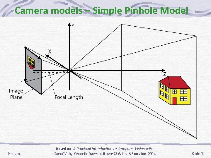
Camera models – Simple Pinhole Model Images Based on A Practical Introduction to Computer Vision with Open. CV by Kenneth Dawson-Howe © Wiley & Sons Inc. 2014 Slide 3

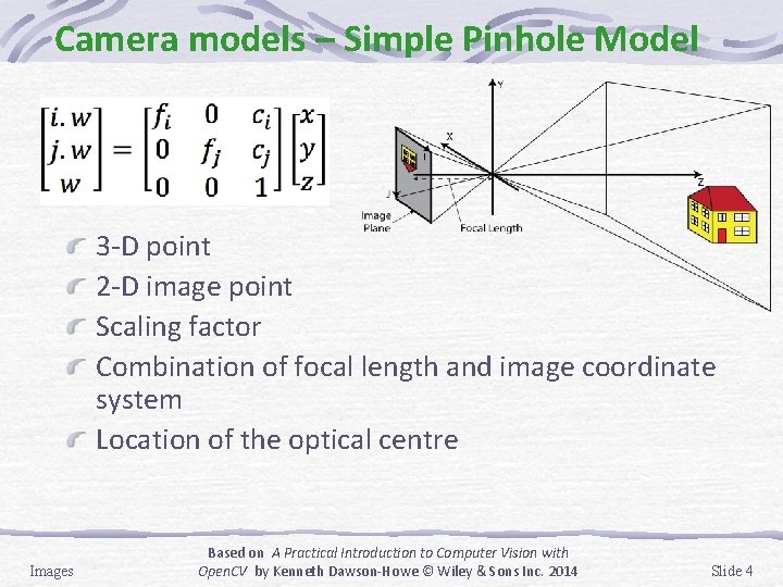
Camera models – Simple Pinhole Model 3 -D point 2 -D image point Scaling factor Combination of focal length and image coordinate system Location of the optical centre Images Based on A Practical Introduction to Computer Vision with Open. CV by Kenneth Dawson-Howe © Wiley & Sons Inc. 2014 Slide 4

Digital Images Theoretically images are continuous 2 D functions of reflected scene brightness. (i, j) or (column, row) or (x, y) To process on a computer we need a discrete representation Sample Quantise Images Based on A Practical Introduction to Computer Vision with Open. CV by Kenneth Dawson-Howe © Wiley & Sons Inc. 2014 Slide 5

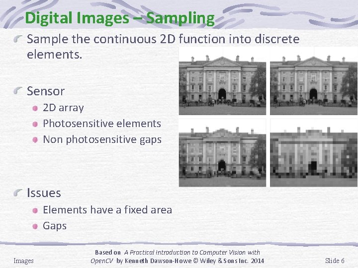
Digital Images – Sampling Sample the continuous 2 D function into discrete elements. Sensor 2 D array Photosensitive elements Non photosensitive gaps Issues Elements have a fixed area Gaps Images Based on A Practical Introduction to Computer Vision with Open. CV by Kenneth Dawson-Howe © Wiley & Sons Inc. 2014 Slide 6

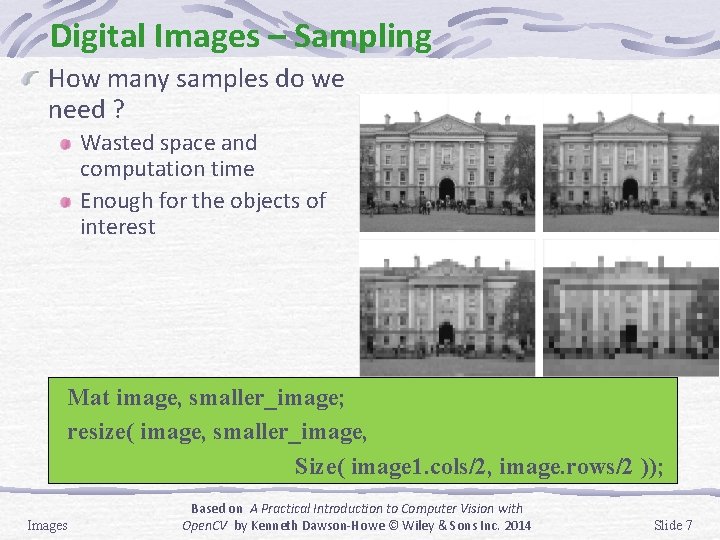
Digital Images – Sampling How many samples do we need ? Wasted space and computation time Enough for the objects of interest Mat image, smaller_image; resize( image, smaller_image, Size( image 1. cols/2, image. rows/2 )); Images Based on A Practical Introduction to Computer Vision with Open. CV by Kenneth Dawson-Howe © Wiley & Sons Inc. 2014 Slide 7

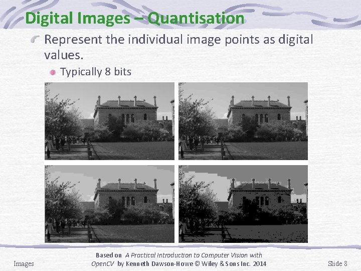
Digital Images – Quantisation Represent the individual image points as digital values. Typically 8 bits Images Based on A Practical Introduction to Computer Vision with Open. CV by Kenneth Dawson-Howe © Wiley & Sons Inc. 2014 Slide 8

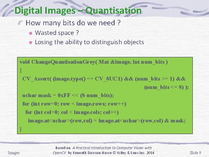
Digital Images – Quantisation How many bits do we need ? Wasted space ? Losing the ability to distinguish objects void Change. Quantisation. Grey( Mat &image, int num_bits ) { CV_Assert( (image. type() == CV_8 UC 1) && (num_bits >= 1) && (num_bits <= 8) ); uchar mask = 0 x. FF << (8 -num_bits); for (int row=0; row < image. rows; row++) for (int col=0; col < image. cols; col++) image. at<uchar>(row, col) = image. at<uchar>(row, col) & mask; } Images Based on A Practical Introduction to Computer Vision with Open. CV by Kenneth Dawson-Howe © Wiley & Sons Inc. 2014 Slide 9

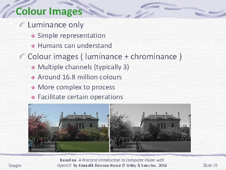
Colour Images Luminance only Simple representation Humans can understand Colour images ( luminance + chrominance ) Multiple channels (typically 3) Around 16. 8 million colours More complex to process Facilitate certain operations Images Based on A Practical Introduction to Computer Vision with Open. CV by Kenneth Dawson-Howe © Wiley & Sons Inc. 2014 Slide 10

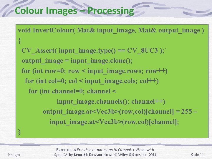
Colour Images – Processing void Invert. Colour( Mat& input_image, Mat& output_image ) { CV_Assert( input_image. type() == CV_8 UC 3 ); ` output_image = input_image. clone(); for (int row=0; row < input_image. rows; row++) for (int col=0; col < input_image. cols; col++) for (int channel=0; channel < input_image. channels(); channel++) output_image. at<Vec 3 b>(row, col)[channel] = 255 – input_image. at<Vec 3 b>(row, col)[channel]; } Images Based on A Practical Introduction to Computer Vision with Open. CV by Kenneth Dawson-Howe © Wiley & Sons Inc. 2014 Slide 11

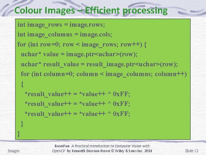
Colour Images – Efficient processing int image_rows = image. rows; int image_columns = image. cols; for (int row=0; row < image_rows; row++) { uchar* value = image. ptr<uchar>(row); uchar* result_value = result_image. ptr<uchar>(row); for (int column=0; column < image_columns; column++) { *result_value++ = *value++ ^ 0 x. FF; } } Images Based on A Practical Introduction to Computer Vision with Open. CV by Kenneth Dawson-Howe © Wiley & Sons Inc. 2014 Slide 12

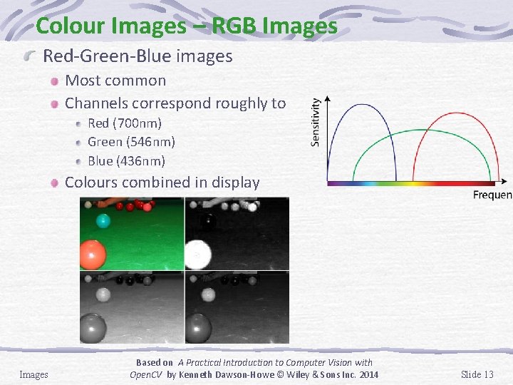
Colour Images – RGB Images Red-Green-Blue images Most common Channels correspond roughly to Red (700 nm) Green (546 nm) Blue (436 nm) Colours combined in display Images Based on A Practical Introduction to Computer Vision with Open. CV by Kenneth Dawson-Howe © Wiley & Sons Inc. 2014 Slide 13

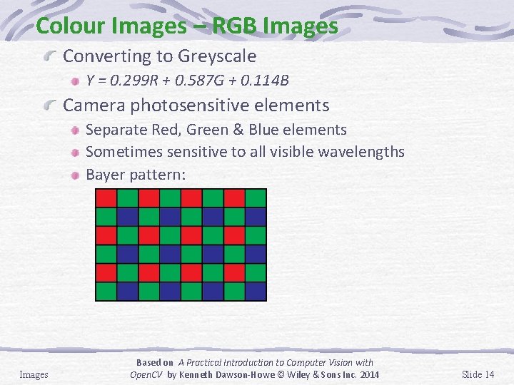
Colour Images – RGB Images Converting to Greyscale Y = 0. 299 R + 0. 587 G + 0. 114 B Camera photosensitive elements Separate Red, Green & Blue elements Sometimes sensitive to all visible wavelengths Bayer pattern: Images Based on A Practical Introduction to Computer Vision with Open. CV by Kenneth Dawson-Howe © Wiley & Sons Inc. 2014 Slide 14

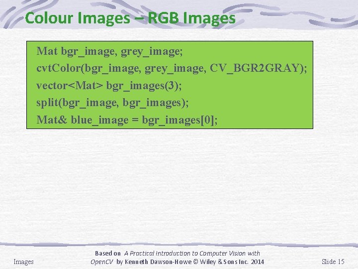
Colour Images – RGB Images Mat bgr_image, grey_image; cvt. Color(bgr_image, grey_image, CV_BGR 2 GRAY); vector<Mat> bgr_images(3); split(bgr_image, bgr_images); Mat& blue_image = bgr_images[0]; Images Based on A Practical Introduction to Computer Vision with Open. CV by Kenneth Dawson-Howe © Wiley & Sons Inc. 2014 Slide 15

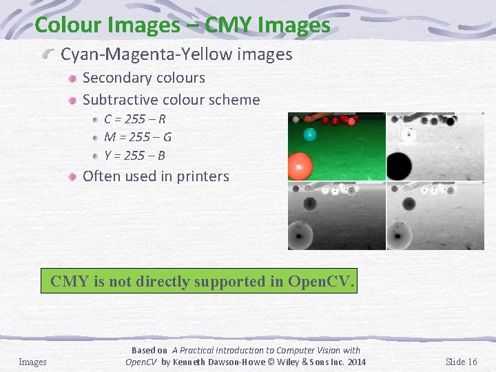
Colour Images – CMY Images Cyan-Magenta-Yellow images Secondary colours Subtractive colour scheme C = 255 – R M = 255 – G Y = 255 – B Often used in printers CMY is not directly supported in Open. CV. Images Based on A Practical Introduction to Computer Vision with Open. CV by Kenneth Dawson-Howe © Wiley & Sons Inc. 2014 Slide 16

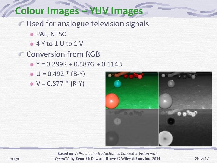
Colour Images – YUV Images Used for analogue television signals PAL, NTSC 4 Y to 1 U to 1 V Conversion from RGB Y = 0. 299 R + 0. 587 G + 0. 114 B U = 0. 492 * (B-Y) V = 0. 877 * (R-Y) Images Based on A Practical Introduction to Computer Vision with Open. CV by Kenneth Dawson-Howe © Wiley & Sons Inc. 2014 Slide 17

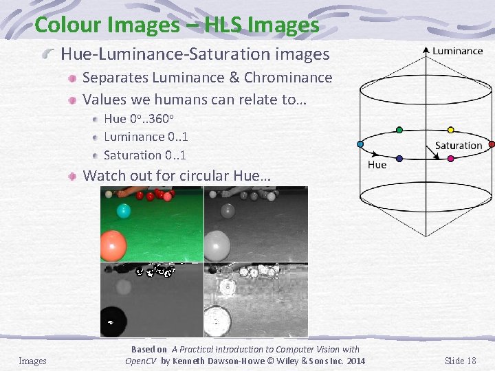
Colour Images – HLS Images Hue-Luminance-Saturation images Separates Luminance & Chrominance Values we humans can relate to… Hue 0 o. . 360 o Luminance 0. . 1 Saturation 0. . 1 Watch out for circular Hue… Images Based on A Practical Introduction to Computer Vision with Open. CV by Kenneth Dawson-Howe © Wiley & Sons Inc. 2014 Slide 18

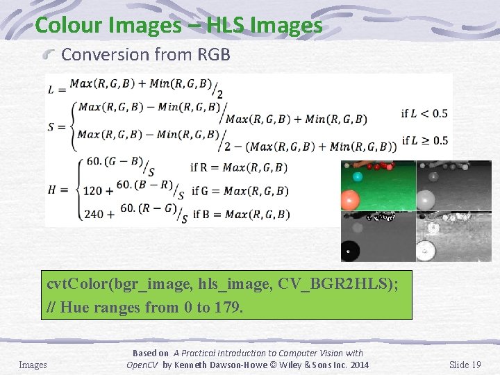
Colour Images – HLS Images Conversion from RGB cvt. Color(bgr_image, hls_image, CV_BGR 2 HLS); // Hue ranges from 0 to 179. Images Based on A Practical Introduction to Computer Vision with Open. CV by Kenneth Dawson-Howe © Wiley & Sons Inc. 2014 Slide 19

Colour Images – Other colour spaces HSV YCr. Cb CIE XYZ CIE L*u*v* CIE L*a*b* Bayer Images Based on A Practical Introduction to Computer Vision with Open. CV by Kenneth Dawson-Howe © Wiley & Sons Inc. 2014 Slide 20

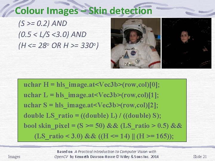
Colour Images – Skin detection (S >= 0. 2) AND (0. 5 < L/S <3. 0) AND (H <= 28 o OR H >= 330 o) uchar H = hls_image. at<Vec 3 b>(row, col)[0]; uchar L = hls_image. at<Vec 3 b>(row, col)[1]; uchar S = hls_image. at<Vec 3 b>(row, col)[2]; double LS_ratio = ((double) L) / ((double) S); bool skin_pixel = (S >= 50) && (LS_ratio > 0. 5) && (LS_ratio < 3. 0) && ((H <= 14) || (H >= 165)); Images Based on A Practical Introduction to Computer Vision with Open. CV by Kenneth Dawson-Howe © Wiley & Sons Inc. 2014 Slide 21

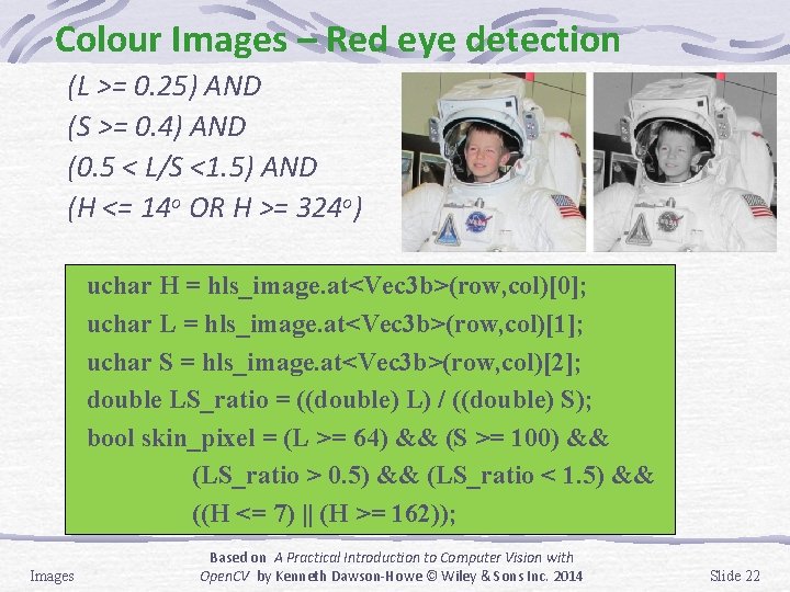
Colour Images – Red eye detection (L >= 0. 25) AND (S >= 0. 4) AND (0. 5 < L/S <1. 5) AND (H <= 14 o OR H >= 324 o) uchar H = hls_image. at<Vec 3 b>(row, col)[0]; uchar L = hls_image. at<Vec 3 b>(row, col)[1]; uchar S = hls_image. at<Vec 3 b>(row, col)[2]; double LS_ratio = ((double) L) / ((double) S); bool skin_pixel = (L >= 64) && (S >= 100) && (LS_ratio > 0. 5) && (LS_ratio < 1. 5) && ((H <= 7) || (H >= 162)); Images Based on A Practical Introduction to Computer Vision with Open. CV by Kenneth Dawson-Howe © Wiley & Sons Inc. 2014 Slide 22

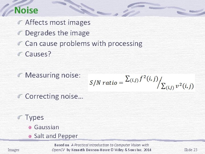
Noise Affects most images Degrades the image Can cause problems with processing Causes? Measuring noise: Correcting noise… Types Gaussian Salt and Pepper Images Based on A Practical Introduction to Computer Vision with Open. CV by Kenneth Dawson-Howe © Wiley & Sons Inc. 2014 Slide 23

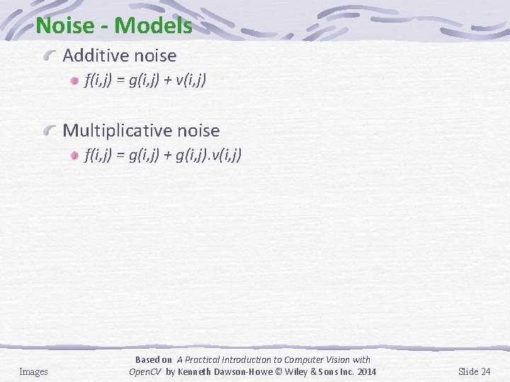
Noise - Models Additive noise f(i, j) = g(i, j) + v(i, j) Multiplicative noise f(i, j) = g(i, j) + g(i, j). v(i, j) Images Based on A Practical Introduction to Computer Vision with Open. CV by Kenneth Dawson-Howe © Wiley & Sons Inc. 2014 Slide 24

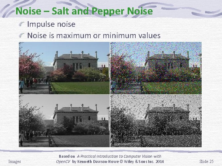
Noise – Salt and Pepper Noise Impulse noise Noise is maximum or minimum values Images Based on A Practical Introduction to Computer Vision with Open. CV by Kenneth Dawson-Howe © Wiley & Sons Inc. 2014 Slide 25

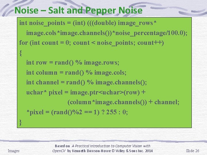
Noise – Salt and Pepper Noise int noise_points = (int) (((double) image_rows* image. cols*image. channels())*noise_percentage/100. 0); for (int count = 0; count < noise_points; count++) { int row = rand() % image. rows; int column = rand() % image. cols; int channel = rand() % image. channels(); uchar* pixel = image. ptr<uchar>(row) + (column*image. channels()) + channel; *pixel = (rand()%2 == 1) ? 255 : 0; } Images Based on A Practical Introduction to Computer Vision with Open. CV by Kenneth Dawson-Howe © Wiley & Sons Inc. 2014 Slide 26

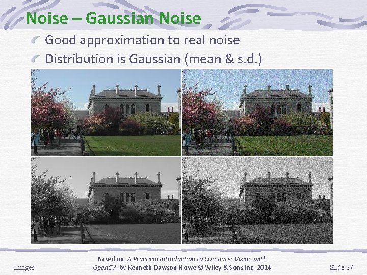
Noise – Gaussian Noise Good approximation to real noise Distribution is Gaussian (mean & s. d. ) Images Based on A Practical Introduction to Computer Vision with Open. CV by Kenneth Dawson-Howe © Wiley & Sons Inc. 2014 Slide 27

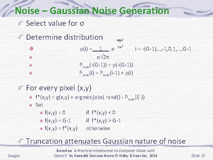
Noise – Gaussian Noise Generation Select value for σ Determine distribution p(i) = -(i)2 2σ2 1. e i = -(G-1), . . , -1, 0, 1, …, G-1 σ 2 Pcum(-(G-1)) = p(-(G-1)) Pcum(i) = Pcum(i-1) + p(i) For every pixel (x, y) f*(x, y) = g(x, y) + argmini(abs( rand() - Pcum[i] )) Set f(x, y) = 0 if f*(x, y) < 0 f(x, y) = G-1 if f*(x, y) > G-1 f(x, y) = f*(x, y) otherwise Truncation attenuates Gaussian nature of noise Images Based on A Practical Introduction to Computer Vision with Open. CV by Kenneth Dawson-Howe © Wiley & Sons Inc. 2014 Slide 28

Noise – Gaussian Noise Mat noise_image(image. size(), CV_16 SC 3); randn(noise_image, Scalar: : all(average), Scalar: : all(standard_deviation)); Mat temp_image; image. convert. To(temp_image, CV_16 SC 3); add. Weighted(temp_image, 1. 0, noise_image, 1. 0, 0. 0, temp_image); temp_image. convert. To(image, image. type()); Images Based on A Practical Introduction to Computer Vision with Open. CV by Kenneth Dawson-Howe © Wiley & Sons Inc. 2014 Slide 29

Smoothing Removing or reducing noise… Linear smoothing transformations Image Averaging Local Averaging Gaussian Smoothing Non-linear transformations Rotating Mask Median Filter Images Based on A Practical Introduction to Computer Vision with Open. CV by Kenneth Dawson-Howe © Wiley & Sons Inc. 2014 Slide 30

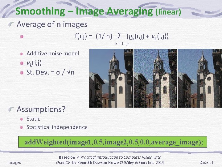
Smoothing – Image Averaging (linear) Average of n images f(i, j) = (1/ n). Σ (gk(i, j) + vk(i, j)) k = 1. . , n Additive noise model vk(i, j) St. Dev. = σ / n Assumptions? Static Statistical independence add. Weighted(image 1, 0. 5, image 2, 0. 5, 0. 0, average_image); Images Based on A Practical Introduction to Computer Vision with Open. CV by Kenneth Dawson-Howe © Wiley & Sons Inc. 2014 Slide 31

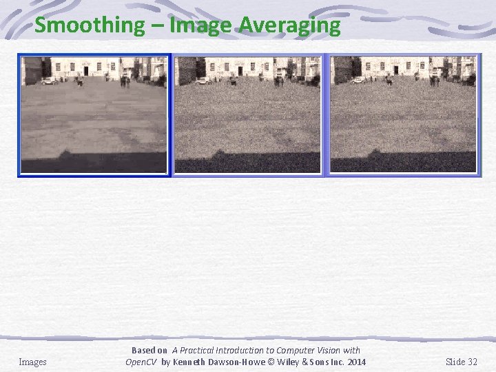
Smoothing – Image Averaging Images Based on A Practical Introduction to Computer Vision with Open. CV by Kenneth Dawson-Howe © Wiley & Sons Inc. 2014 Slide 32

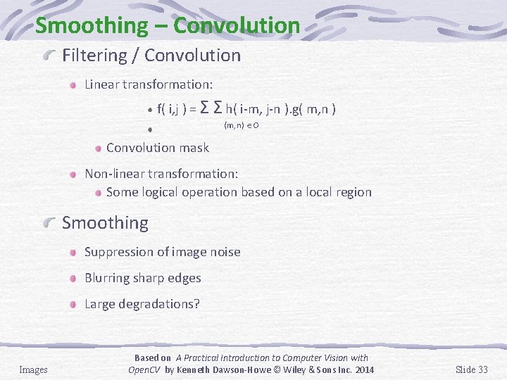
Smoothing – Convolution Filtering / Convolution Linear transformation: f( i, j ) = Σ Σ h( i-m, j-n ). g( m, n ) (m, n) Ο Convolution mask Non-linear transformation: Some logical operation based on a local region Smoothing Suppression of image noise Blurring sharp edges Large degradations? Images Based on A Practical Introduction to Computer Vision with Open. CV by Kenneth Dawson-Howe © Wiley & Sons Inc. 2014 Slide 33

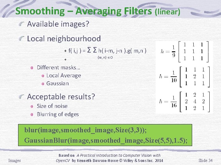
Smoothing – Averaging Filters (linear) Available images? Local neighbourhood f( i, j ) = Σ Σ h( i-m, j-n ). g( m, n ) (m, n) Ο Different masks… Local Average Gaussian Acceptable results? Size of noise Blurring of edges blur(image, smoothed_image, Size(3, 3)); Gaussian. Blur(image, smoothed_image, Size(5, 5), 1. 5); Images Based on A Practical Introduction to Computer Vision with Open. CV by Kenneth Dawson-Howe © Wiley & Sons Inc. 2014 Slide 34

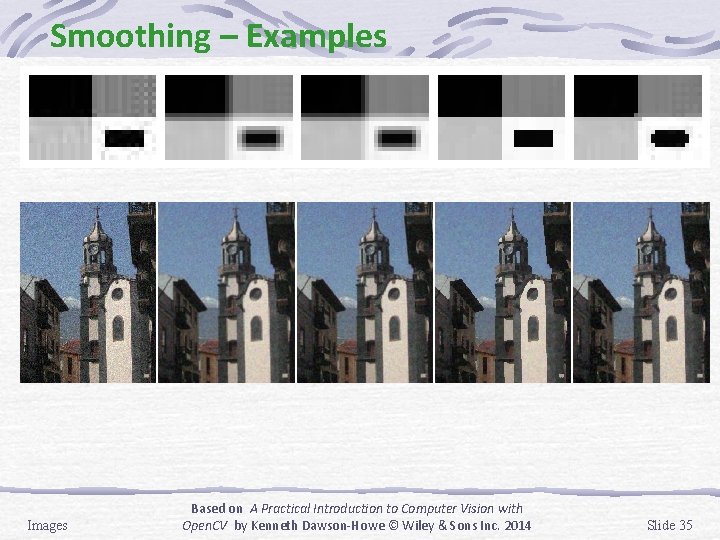
Smoothing – Examples Images Based on A Practical Introduction to Computer Vision with Open. CV by Kenneth Dawson-Howe © Wiley & Sons Inc. 2014 Slide 35

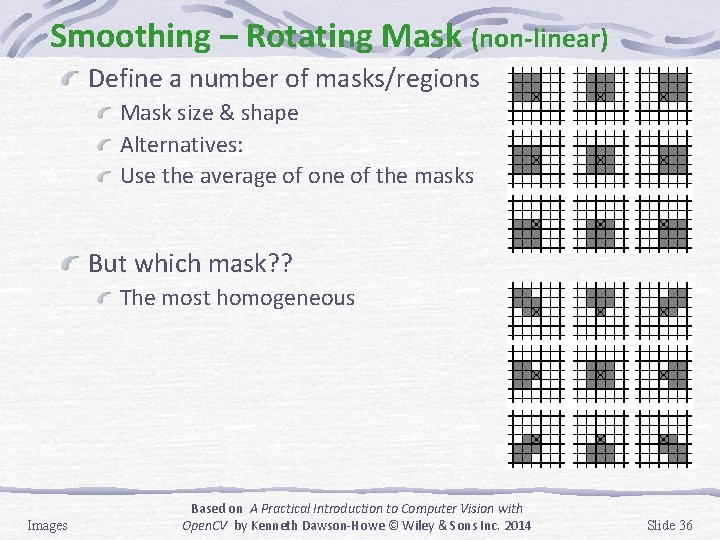
Smoothing – Rotating Mask (non-linear) Define a number of masks/regions Mask size & shape Alternatives: Use the average of one of the masks But which mask? ? The most homogeneous Images Based on A Practical Introduction to Computer Vision with Open. CV by Kenneth Dawson-Howe © Wiley & Sons Inc. 2014 Slide 36

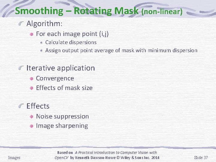
Smoothing – Rotating Mask (non-linear) Algorithm: For each image point (i, j) Calculate dispersions Assign output point average of mask with minimum dispersion Iterative application Convergence Effects of mask size Effects Noise suppression Image sharpening Images Based on A Practical Introduction to Computer Vision with Open. CV by Kenneth Dawson-Howe © Wiley & Sons Inc. 2014 Slide 37

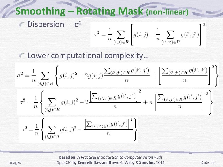
Smoothing – Rotating Mask (non-linear) Dispersion σ2 Lower computational complexity… Images Based on A Practical Introduction to Computer Vision with Open. CV by Kenneth Dawson-Howe © Wiley & Sons Inc. 2014 Slide 38

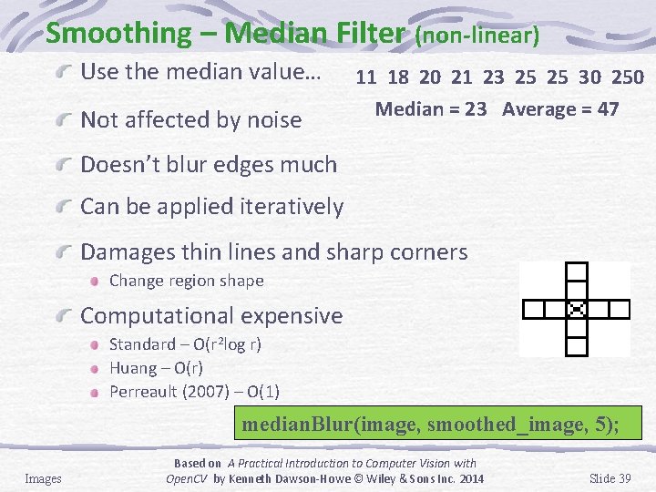
Smoothing – Median Filter (non-linear) Use the median value… Not affected by noise 11 18 20 21 23 25 25 30 250 Median = 23 Average = 47 Doesn’t blur edges much Can be applied iteratively Damages thin lines and sharp corners Change region shape Computational expensive Standard – O(r 2 log r) Huang – O(r) Perreault (2007) – O(1) median. Blur(image, smoothed_image, 5); Images Based on A Practical Introduction to Computer Vision with Open. CV by Kenneth Dawson-Howe © Wiley & Sons Inc. 2014 Slide 39

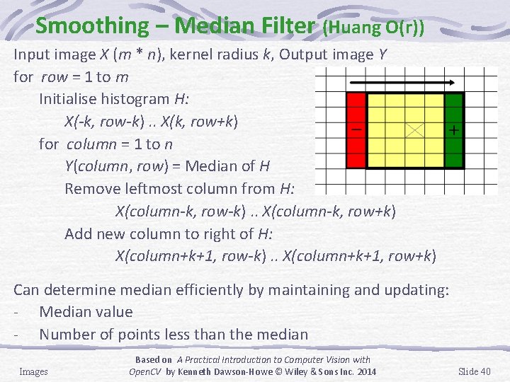
Smoothing – Median Filter (Huang O(r)) Input image X (m * n), kernel radius k, Output image Y for row = 1 to m Initialise histogram H: X(-k, row-k). . X(k, row+k) for column = 1 to n Y(column, row) = Median of H Remove leftmost column from H: X(column-k, row-k). . X(column-k, row+k) Add new column to right of H: X(column+k+1, row-k). . X(column+k+1, row+k) Can determine median efficiently by maintaining and updating: - Median value - Number of points less than the median Images Based on A Practical Introduction to Computer Vision with Open. CV by Kenneth Dawson-Howe © Wiley & Sons Inc. 2014 Slide 40

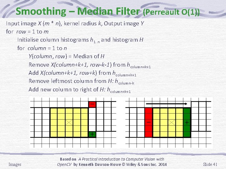
Smoothing – Median Filter (Perreault O(1)) Input image X (m * n), kernel radius k, Output image Y for row = 1 to m Initialise column histograms h 1. . n and histogram H for column = 1 to n Y(column, row) = Median of H Remove X(column+k+1, row-k-1) from hcolumn+k+1 Add X(column+k+1, row+k) from hcolumn+k+1 Remove leftmost column from H: hcolumn-k Add new column to right of H: hcolumn+k+1 Images Based on A Practical Introduction to Computer Vision with Open. CV by Kenneth Dawson-Howe © Wiley & Sons Inc. 2014 Slide 41

Smoothing – Examples Images Based on A Practical Introduction to Computer Vision with Open. CV by Kenneth Dawson-Howe © Wiley & Sons Inc. 2014 Slide 42