Image SuperResolution as Sparse Representation of Raw Image

Image Super-Resolution as Sparse Representation of Raw Image Patches Jianchao Yang, John Wright, Thomas Huang, Yi Ma CVPR 2008

Outline �Introduction �Super-resolution from Sparsity �Local Model from Sparse Representation �Enforcing Global Reconstruction Constraint �Global Optimization Interpretation �Dictionary Preparation �Experiments �Discussion 2

Introduction �To generate a super-resolution (SR) image requires multiple low-resolution images of the same scene, typically aligned with sub-pixel accuracy �MAP (maximum a-posteriori) �Markov Random Field (MRF) solved by belief propagation �Bilateral Total Variation �The SR task is cast as the inverse problem of recovering the original high-resolution image by fusing the low-resolution images 3

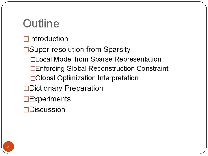
Introduction �Let be an overcomplete dictionary of K prototype signal-atoms �Suppose a signal can be represented as a sparse linear combination of these atoms �The signal vector can be written as , where is a vector with very few (<<K) nonzero entries �In practice, we might observe only a small set of measurements of : where 4 with

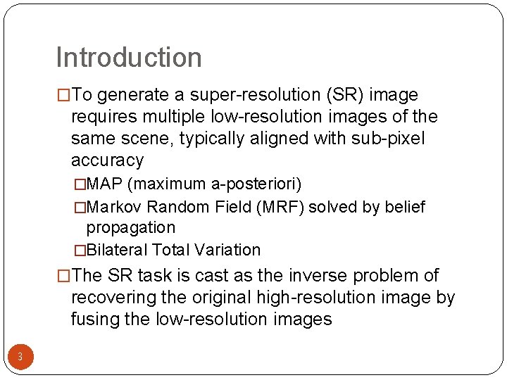
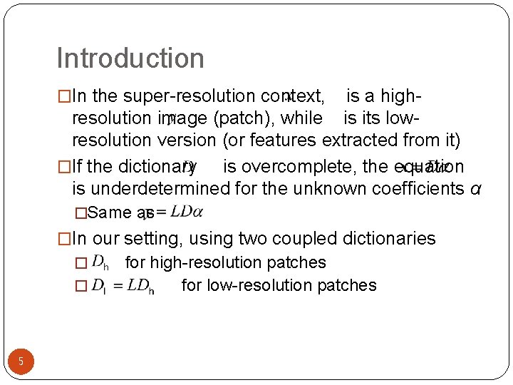
Introduction �In the super-resolution context, is a highresolution image (patch), while is its lowresolution version (or features extracted from it) �If the dictionary is overcomplete, the equation is underdetermined for the unknown coefficients α �Same as �In our setting, using two coupled dictionaries � � 5 for high-resolution patches for low-resolution patches

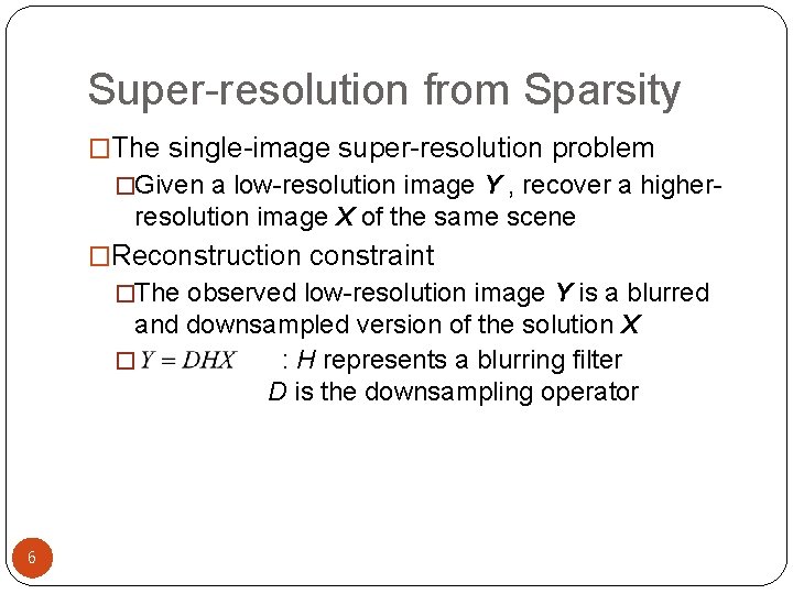
Super-resolution from Sparsity �The single-image super-resolution problem �Given a low-resolution image Y , recover a higher- resolution image X of the same scene �Reconstruction constraint �The observed low-resolution image Y is a blurred and downsampled version of the solution X � : H represents a blurring filter D is the downsampling operator 6

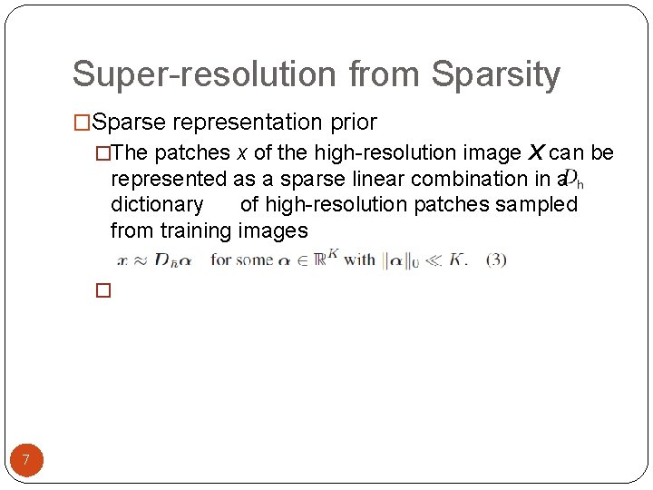
Super-resolution from Sparsity �Sparse representation prior �The patches x of the high-resolution image X can be represented as a sparse linear combination in a dictionary of high-resolution patches sampled from training images � 7

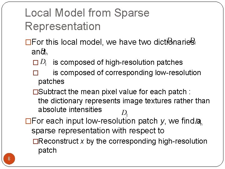
Local Model from Sparse Representation �For this local model, we have two dictionaries and is composed of high-resolution patches � is composed of corresponding low-resolution patches �Subtract the mean pixel value for each patch : the dictionary represents image textures rather than absolute intensities � �For each input low-resolution patch y, we find a sparse representation with respect to �Reconstruct x by the corresponding high-resolution patch 8

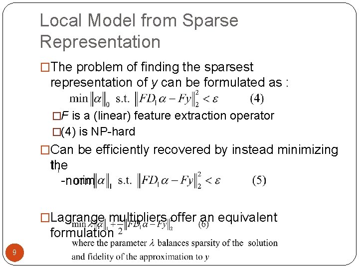
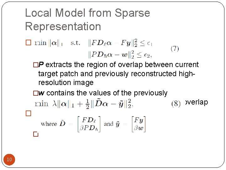
Local Model from Sparse Representation �The problem of finding the sparsest representation of y can be formulated as : �F is a (linear) feature extraction operator �(4) is NP-hard �Can be efficiently recovered by instead minimizing the -norm �Lagrange multipliers offer an equivalent formulation 9

Local Model from Sparse Representation � �P extracts the region of overlap between current target patch and previously reconstructed highresolution image �w contains the values of the previously reconstructed high-resolution image on the overlap � � 10

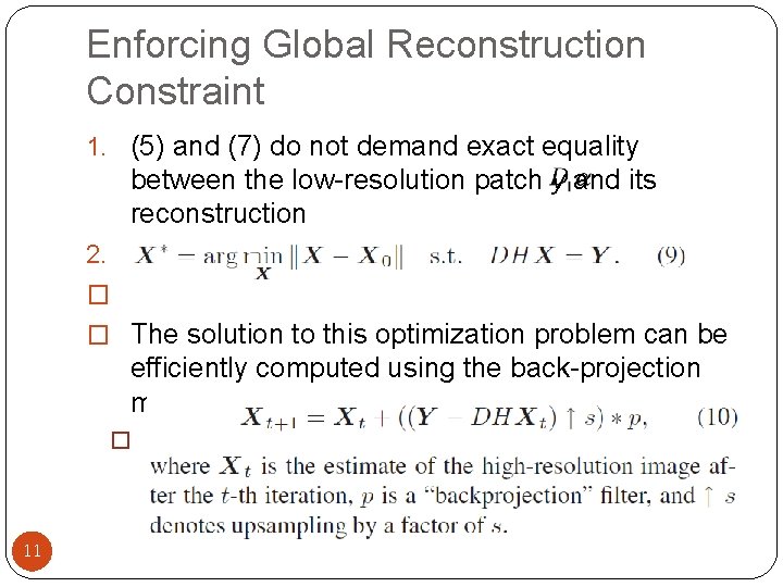
Enforcing Global Reconstruction Constraint 1. (5) and (7) do not demand exact equality between the low-resolution patch y and its reconstruction 2. Because of noise � � The solution to this optimization problem can be efficiently computed using the back-projection method � The update equation for this iterative method is 11

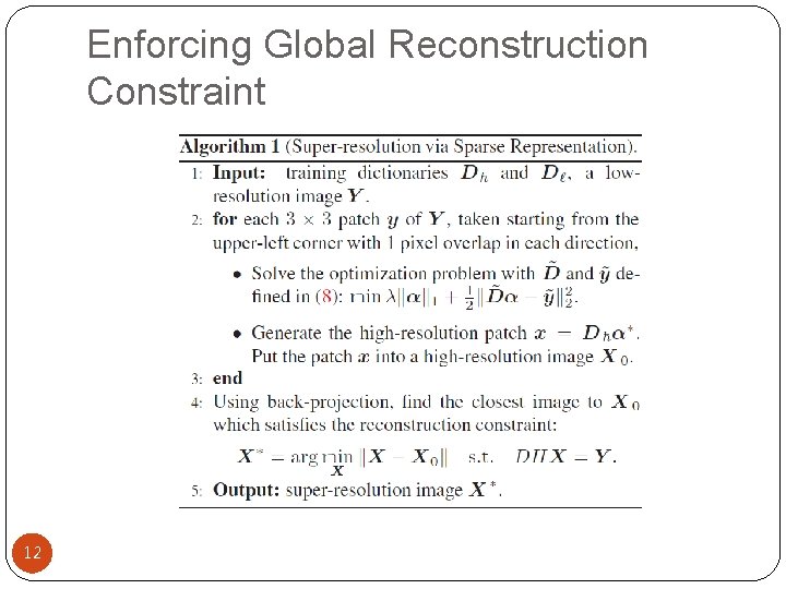
Enforcing Global Reconstruction Constraint 12

Global Optimization Interpretation �Applied image compression, denoising, and restoration [17] �This leads to a large optimization problem 13 [17] J. Mairal, G. Sapiro, and M. Elad. Learning multiscale sparse representations for image and video restoration. SIAM Multiscale Modeling and Simulation, 2008.

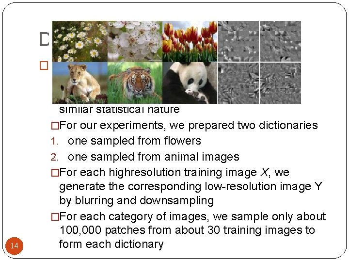
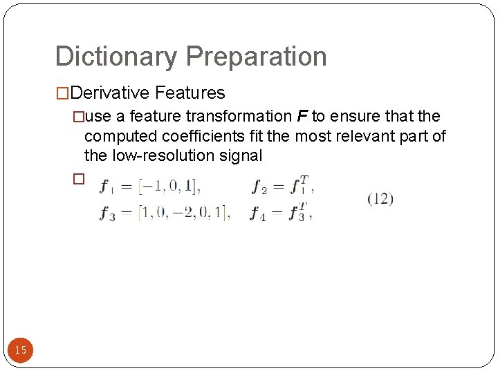
Dictionary Preparation �Random Raw Patches from Training Images �we generate dictionaries by simply randomly 14 sampling raw patches from training images of similar statistical nature �For our experiments, we prepared two dictionaries 1. one sampled from flowers 2. one sampled from animal images �For each highresolution training image X, we generate the corresponding low-resolution image Y by blurring and downsampling �For each category of images, we sample only about 100, 000 patches from about 30 training images to form each dictionary

Dictionary Preparation �Derivative Features �use a feature transformation F to ensure that the computed coefficients fit the most relevant part of the low-resolution signal � 15

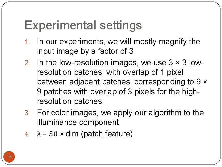
Experimental settings 1. In our experiments, we will mostly magnify the input image by a factor of 3 2. In the low-resolution images, we use 3 × 3 lowresolution patches, with overlap of 1 pixel between adjacent patches, corresponding to 9 × 9 patches with overlap of 3 pixels for the highresolution patches 3. For color images, we apply our algorithm to the illuminance component 4. λ = 50 × dim (patch feature) 16

Experimental results [5] H. Chang, D. -Y. Yeung, and Y. Xiong. Super-resolution through neighbor embedding. CVPR, 2004. 17

Experimental results 18 [6] S. Dai, M. Han, W. Xu, Y. Wu, and Y. Gong. Soft edge smoothness prior for alpha channel super resolution. Proc. ICCV, 2007.

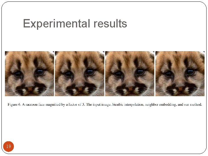
Experimental results 19

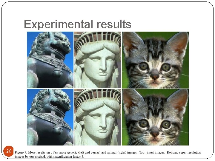
Experimental results 20

Experimental results [12] W. T. Freeman, E. C. Pasztor, and O. T. Carmichael. Learning low-level vision. IJCV, 2000. 21

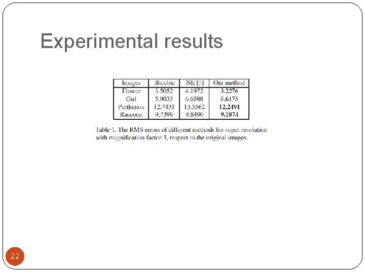
Experimental results 22

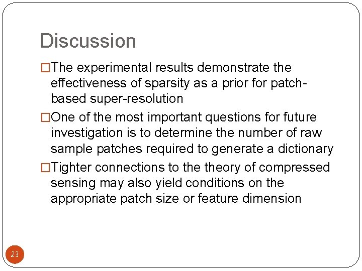
Discussion �The experimental results demonstrate the effectiveness of sparsity as a prior for patchbased super-resolution �One of the most important questions for future investigation is to determine the number of raw sample patches required to generate a dictionary �Tighter connections to theory of compressed sensing may also yield conditions on the appropriate patch size or feature dimension 23