Image Stitching Add example Computer Vision JiaBin Huang

Image Stitching Add example Computer Vision Jia-Bin Huang, Virginia Tech Many slides from S. Seitz and D. Hoiem

Administrative stuffs • HW 3 is out due 11: 59 PM Oct 17 • Please start early. Deadlines are firm. • No emails requesting extensions • Getting help? • *Five* free late days without penalty • Piazza • Office hours • No free late dates for final projects

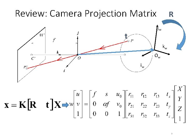
Review: Camera Projection Matrix R jw t kw Ow iw 3

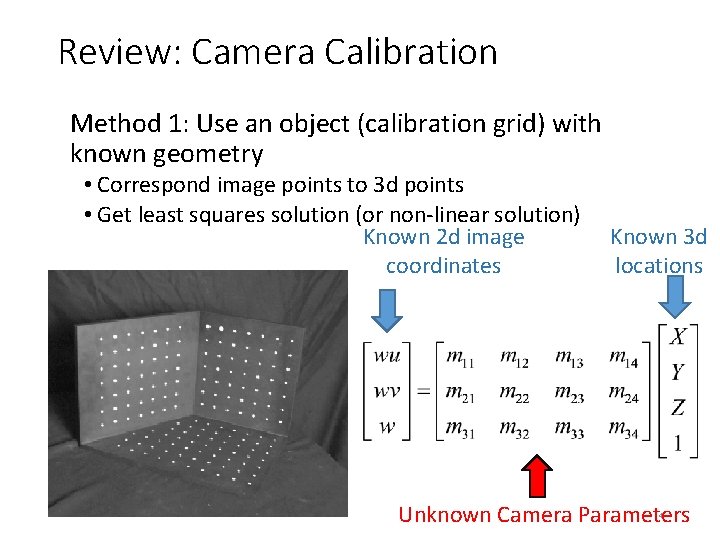
Review: Camera Calibration Method 1: Use an object (calibration grid) with known geometry • Correspond image points to 3 d points • Get least squares solution (or non-linear solution) Known 2 d image coordinates Known 3 d locations Unknown Camera Parameters 4

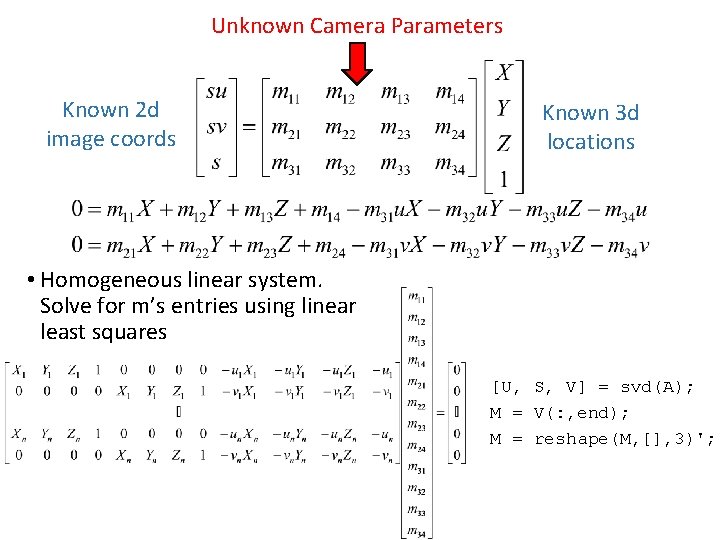
Unknown Camera Parameters Known 2 d image coords Known 3 d locations • Homogeneous linear system. Solve for m’s entries using linear least squares [U, S, V] = svd(A); M = V(: , end); M = reshape(M, [], 3)';

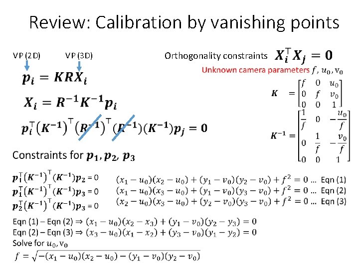
Review: Calibration by vanishing points VP (2 D) • Orthogonality constraints VP (3 D)

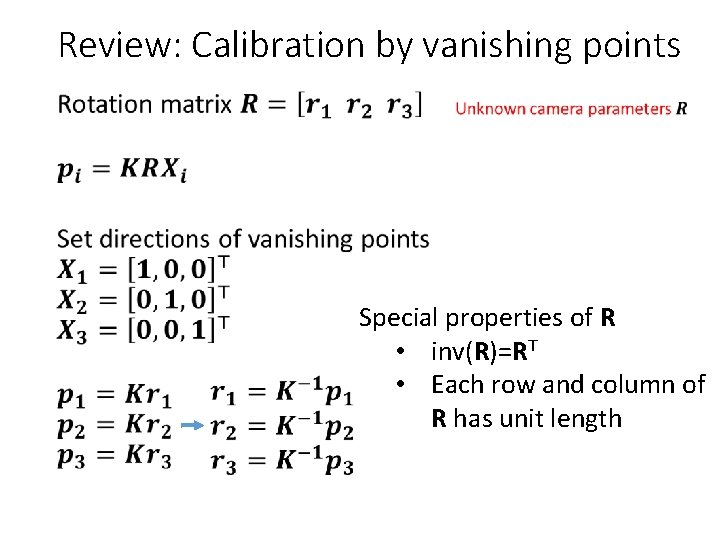
Review: Calibration by vanishing points • Special properties of R • inv(R)=RT • Each row and column of R has unit length

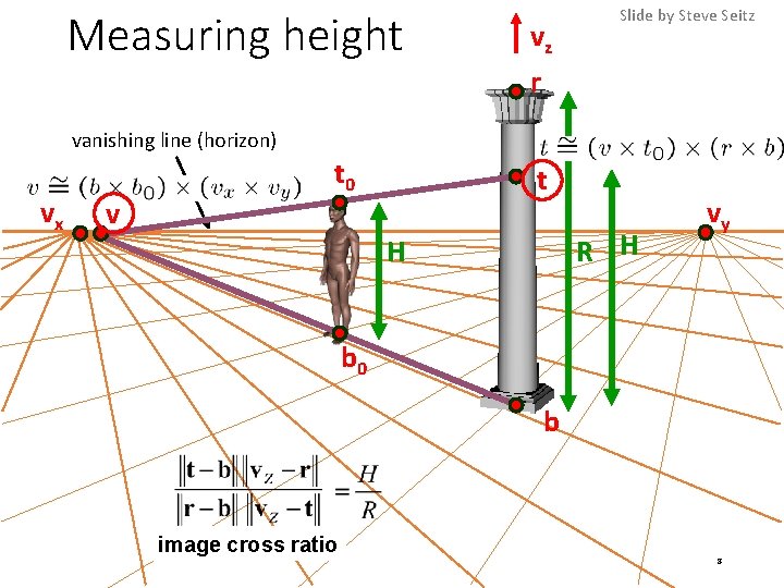
Measuring height vz r Slide by Steve Seitz vanishing line (horizon) vx v t 0 t R H H vy b 0 b image cross ratio 8

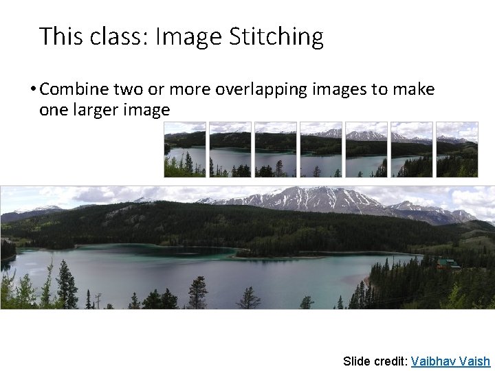
This class: Image Stitching • Combine two or more overlapping images to make one larger image Add example Slide credit: Vaibhav Vaish

Concepts introduced/reviewed in today’s lecture • Camera model • Homographies • Solving homogeneous systems of linear equations • Keypoint-based alignment • RANSAC • Blending • How the iphone stitcher works

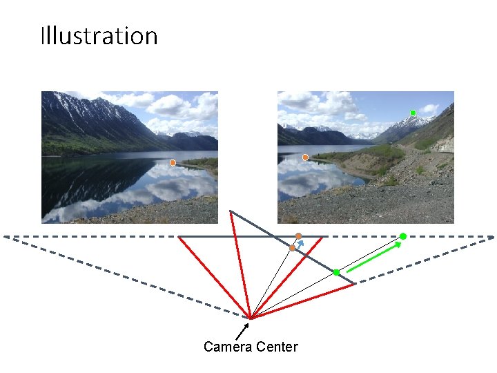
Illustration Camera Center

Problem set-up. X • x = K [R t] X • x' = K' [R' t'] X • t=t'=0 x x' f f' • x'=Hx where H = K' R' R-1 K-1 • Typically only R and f will change (4 parameters), but, in general, H has 8 parameters

Homography • Definition • General mathematics: homography = projective linear transformation • Vision (most common usage): homography = linear transformation between two image planes • Examples • Project 3 D surface into frontal view • Relate two views that differ only by rotation

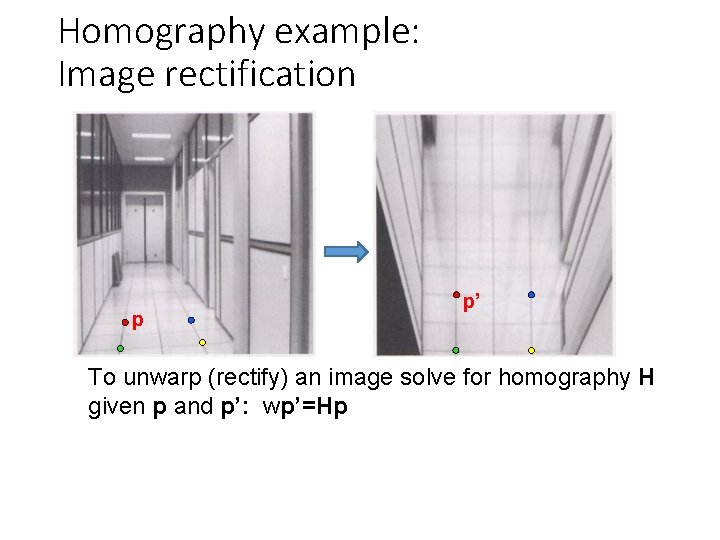
Homography example: Image rectification p p’ To unwarp (rectify) an image solve for homography H given p and p’: wp’=Hp

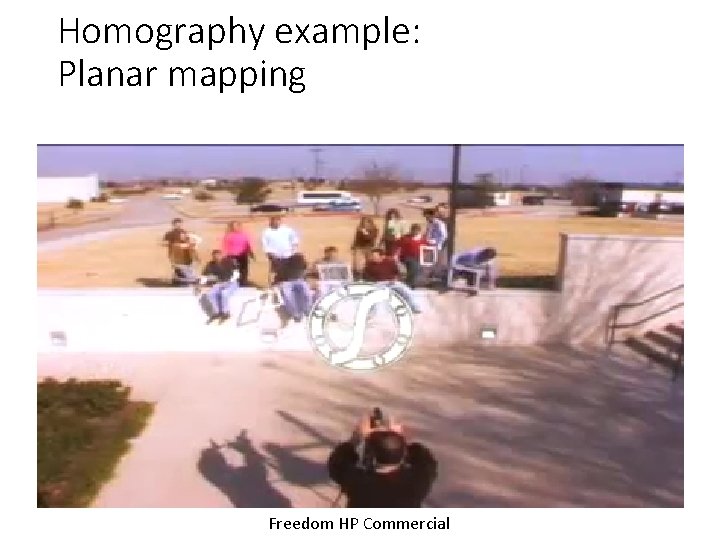
Homography example: Planar mapping Freedom HP Commercial

Image Stitching Algorithm Overview 1. Detect keypoints (e. g. , SIFT) 2. Match keypoints (e. g. , 1 st/2 nd NN < thresh) 3. Estimate homography with four matched keypoints (using RANSAC) 4. Combine images

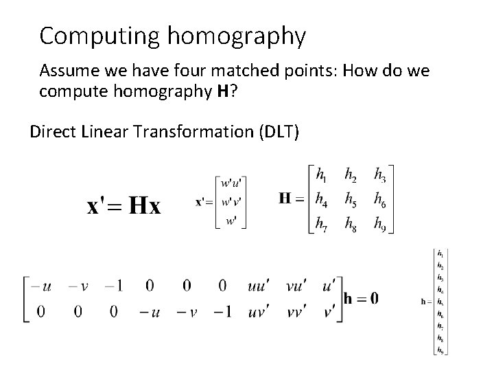
Computing homography Assume we have four matched points: How do we compute homography H? Direct Linear Transformation (DLT)

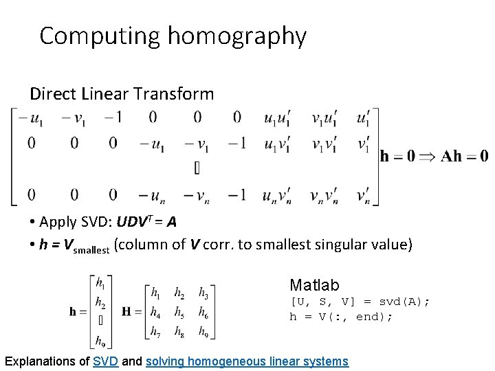
Computing homography Direct Linear Transform • Apply SVD: UDVT = A • h = Vsmallest (column of V corr. to smallest singular value) Matlab [U, S, V] = svd(A); h = V(: , end); Explanations of SVD and solving homogeneous linear systems

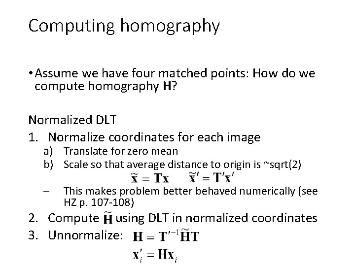
Computing homography • Assume we have four matched points: How do we compute homography H? Normalized DLT 1. Normalize coordinates for each image a) Translate for zero mean b) Scale so that average distance to origin is ~sqrt(2) – This makes problem better behaved numerically (see HZ p. 107 -108) 2. Compute using DLT in normalized coordinates 3. Unnormalize:

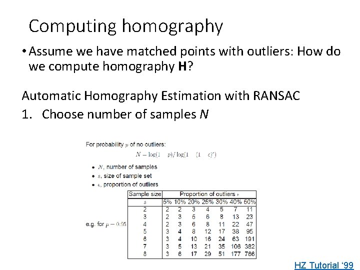
Computing homography • Assume we have matched points with outliers: How do we compute homography H? Automatic Homography Estimation with RANSAC 1. Choose number of samples N HZ Tutorial ‘ 99

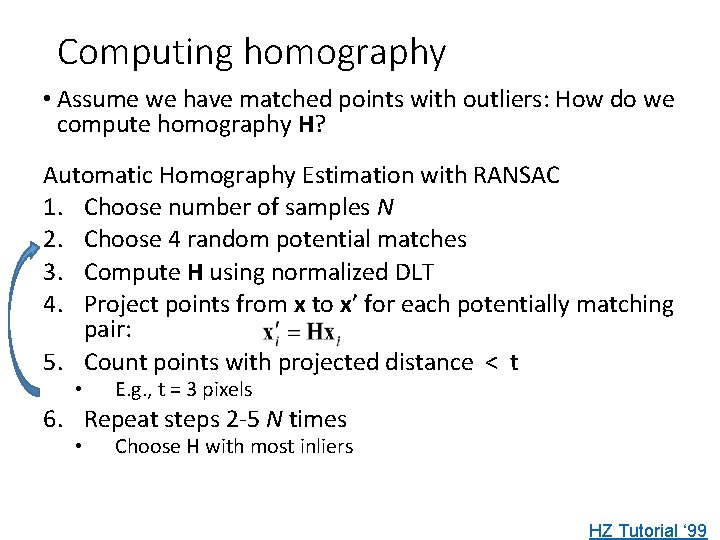
Computing homography • Assume we have matched points with outliers: How do we compute homography H? Automatic Homography Estimation with RANSAC 1. Choose number of samples N 2. Choose 4 random potential matches 3. Compute H using normalized DLT 4. Project points from x to x’ for each potentially matching pair: 5. Count points with projected distance < t • E. g. , t = 3 pixels 6. Repeat steps 2 -5 N times • Choose H with most inliers HZ Tutorial ‘ 99

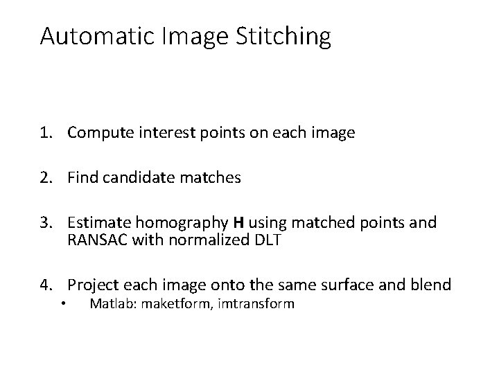
Automatic Image Stitching 1. Compute interest points on each image 2. Find candidate matches 3. Estimate homography H using matched points and RANSAC with normalized DLT 4. Project each image onto the same surface and blend • Matlab: maketform, imtransform

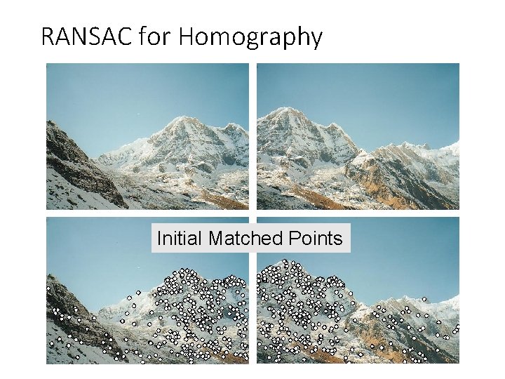
RANSAC for Homography Initial Matched Points

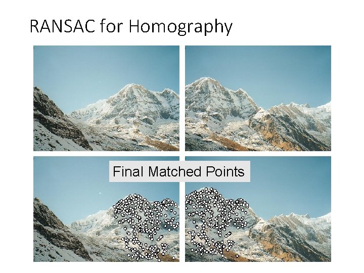
RANSAC for Homography Final Matched Points

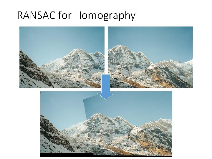
RANSAC for Homography

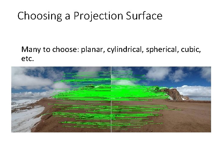
Choosing a Projection Surface Many to choose: planar, cylindrical, spherical, cubic, etc.

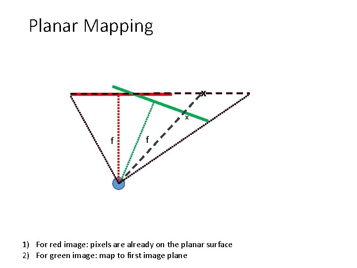
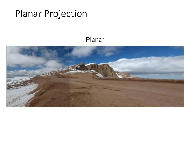
Planar Mapping x x f f 1) For red image: pixels are already on the planar surface 2) For green image: map to first image plane

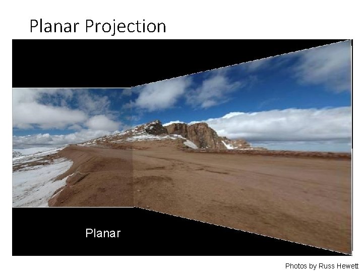
Planar Projection Planar Photos by Russ Hewett

Planar Projection Planar

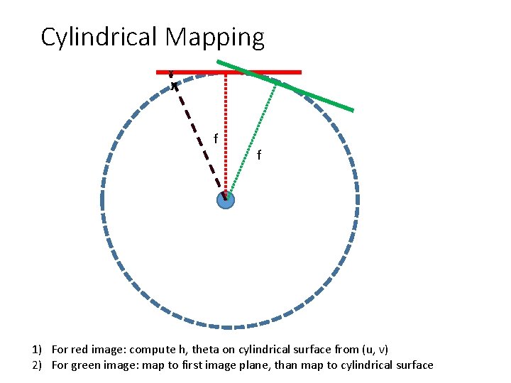
Cylindrical Mapping x x f f 1) For red image: compute h, theta on cylindrical surface from (u, v) 2) For green image: map to first image plane, than map to cylindrical surface

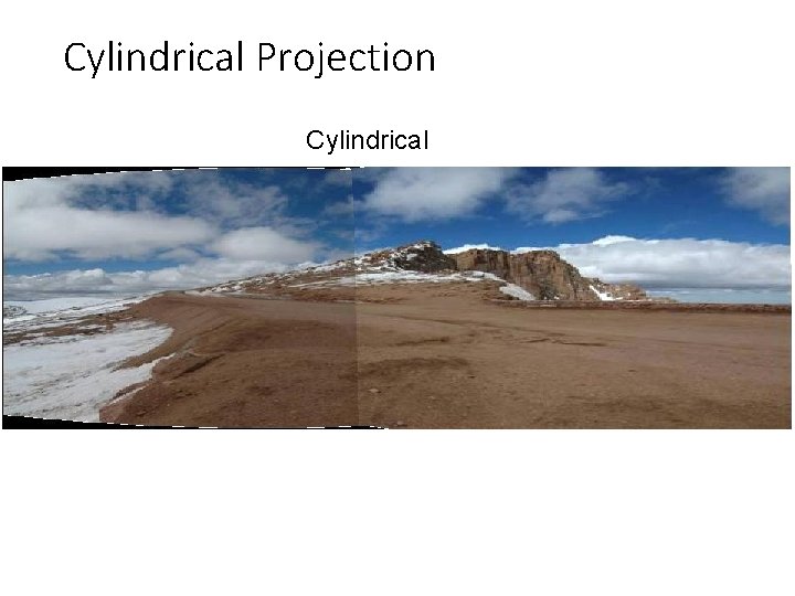
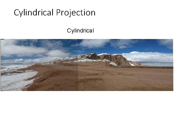
Cylindrical Projection Cylindrical

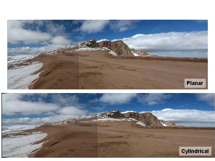
Planar Cylindrical

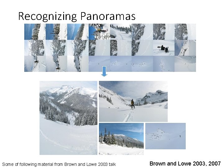
Recognizing Panoramas Some of following material from Brown and Lowe 2003 talk Brown and Lowe 2003, 2007

Recognizing Panoramas Input: N images 1. Extract SIFT points, descriptors from all images 2. Find K-nearest neighbors for each point (K=4) 3. For each image a) Select M candidate matching images by counting matched keypoints (m=6) b) Solve homography Hij for each matched image

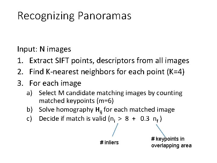
Recognizing Panoramas Input: N images 1. Extract SIFT points, descriptors from all images 2. Find K-nearest neighbors for each point (K=4) 3. For each image a) Select M candidate matching images by counting matched keypoints (m=6) b) Solve homography Hij for each matched image c) Decide if match is valid (ni > 8 + 0. 3 nf ) # inliers # keypoints in overlapping area

Recognizing Panoramas (cont. ) (now we have matched pairs of images) 4. Find connected components

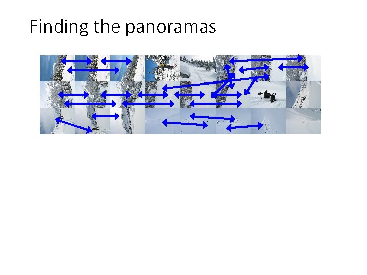
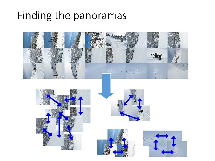
Finding the panoramas

Recognizing Panoramas (cont. ) (now we have matched pairs of images) 4. Find connected components 5. For each connected component a) Perform bundle adjustment to solve for rotation (θ 1, θ 2, θ 3) and focal length f of all cameras b) Project to a surface (plane, cylinder, or sphere) c) Render with multiband blending

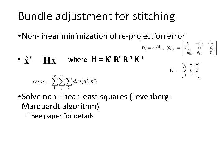
Bundle adjustment for stitching • Non-linear minimization of re-projection error • where H = K’ R’ R-1 K-1 • Solve non-linear least squares (Levenberg. Marquardt algorithm) • See paper for details

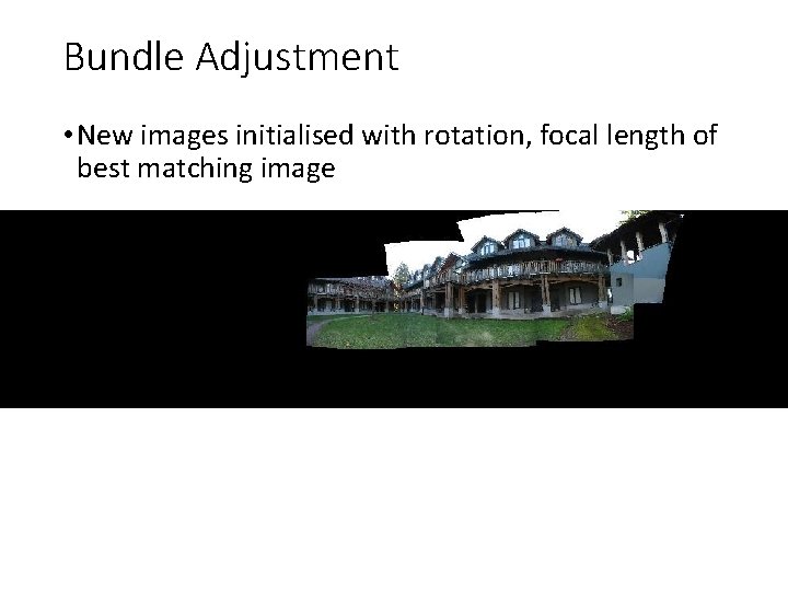
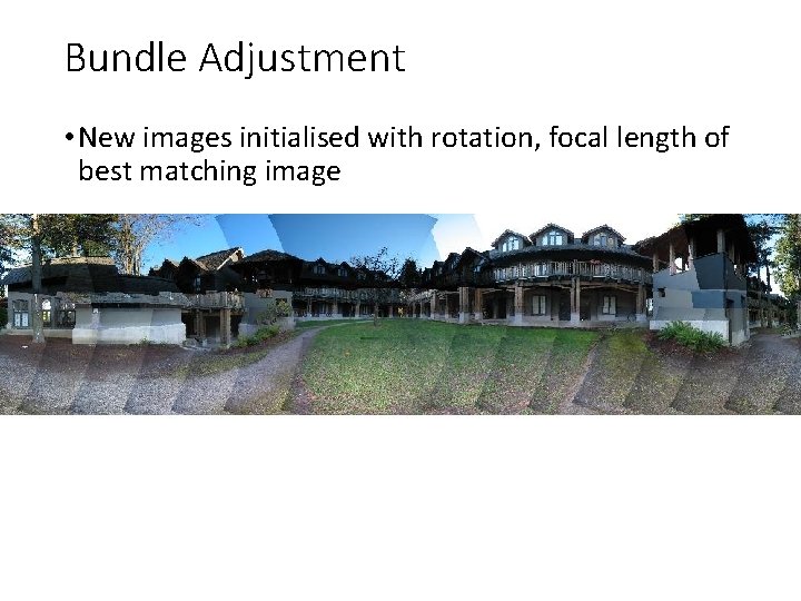
Bundle Adjustment • New images initialised with rotation, focal length of best matching image

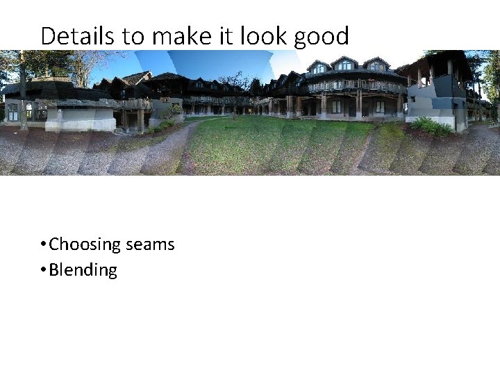
Details to make it look good • Choosing seams • Blending

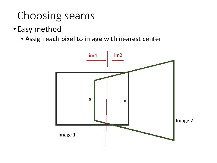
Choosing seams • Easy method • Assign each pixel to image with nearest center im 1 x im 2 x Image 2 Image 1

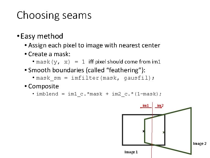
Choosing seams • Easy method • Assign each pixel to image with nearest center • Create a mask: • mask(y, x) = 1 iff pixel should come from im 1 • Smooth boundaries (called “feathering”): • mask_sm = imfilter(mask, gausfil); • Composite • imblend = im 1_c. *mask + im 2_c. *(1 -mask); im 1 x im 2 x Image 2 Image 1

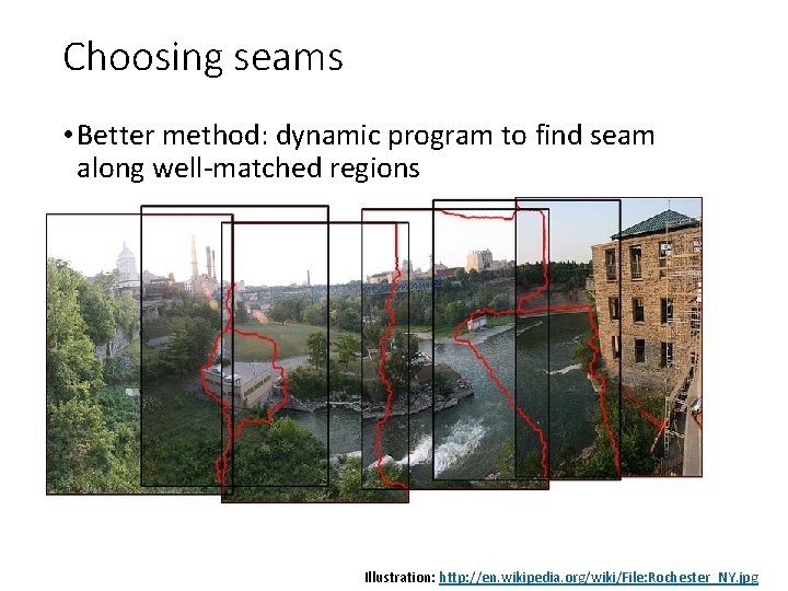
Choosing seams • Better method: dynamic program to find seam along well-matched regions Illustration: http: //en. wikipedia. org/wiki/File: Rochester_NY. jpg

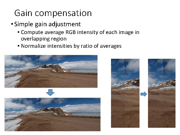
Gain compensation • Simple gain adjustment • Compute average RGB intensity of each image in overlapping region • Normalize intensities by ratio of averages

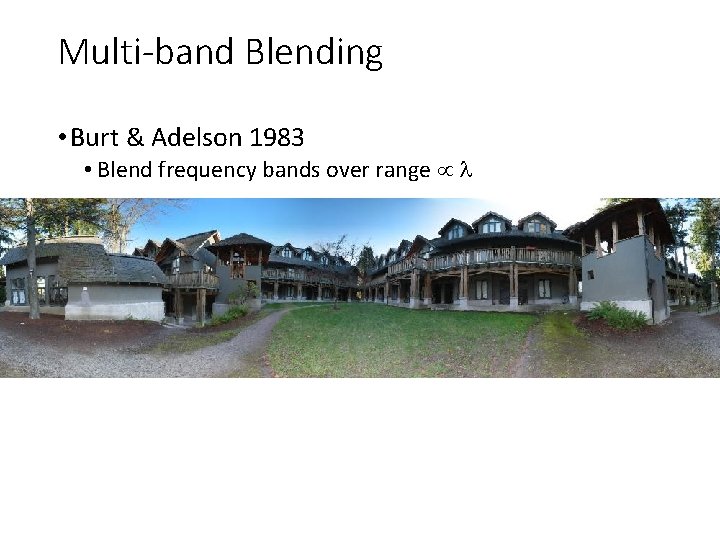
Multi-band Blending • Burt & Adelson 1983 • Blend frequency bands over range l

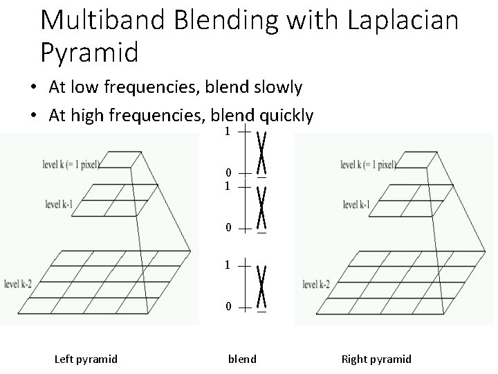
Multiband Blending with Laplacian Pyramid • At low frequencies, blend slowly • At high frequencies, blend quickly 1 0 1 0 Left pyramid blend Right pyramid

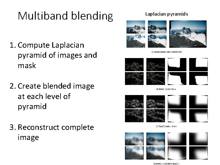
Multiband blending 1. Compute Laplacian pyramid of images and mask 2. Create blended image at each level of pyramid 3. Reconstruct complete image Laplacian pyramids

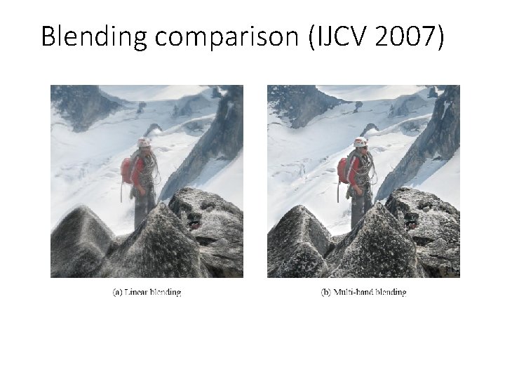
Blending comparison (IJCV 2007)

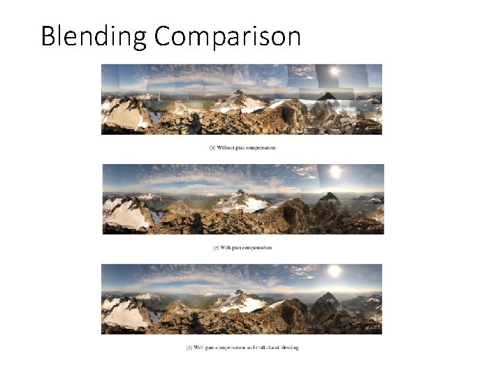
Blending Comparison

Further reading • DLT algorithm: HZ p. 91 (alg 4. 2), p. 585 • Normalization: HZ p. 107 -109 (alg 4. 2) • RANSAC: HZ Sec 4. 7, p. 123, alg 4. 6 • Rick Szeliski’s alignment/stitching tutorial • Recognising Panoramas: Brown and Lowe, IJCV 2007 (also bundle adjustment)

How does iphone panoramic stitching work? • Capture images at 30 fps • Stitch the central 1/8 of a selection of images • Select which images to stitch using the accelerometer and frame-toframe matching • Faster and avoids radial distortion that often occurs towards corners of images • Alignment • Initially, perform cross-correlation of small patches aided by accelerometer to find good regions for matching • Register by matching points (KLT tracking or RANSAC with FAST (similar to SIFT) points) or correlational matching • Blending • Linear (or similar) blending, using a face detector to avoid blurring face regions and choose good face shots (not blinking, etc) http: //www. patentlyapple. com/patently-apple/2012/11/apples-cool-iphone-5 -panorama-app-revealed-in-5 -patents. html

Things to remember • Homography relates rotating cameras • Recover homography using RANSAC and normalized DLT • Bundle adjustment minimizes reprojection error for set of related images • Details to make it look nice (e. g. , blending)

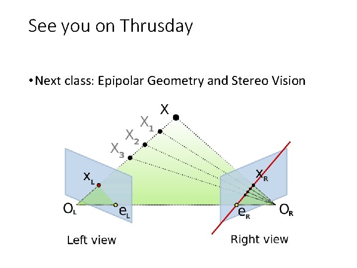
See you on Thrusday • Next class: Epipolar Geometry and Stereo Vision