Image restoration Estimating the degradation function Lecture 11

Image restoration: Estimating the degradation function Lecture 11

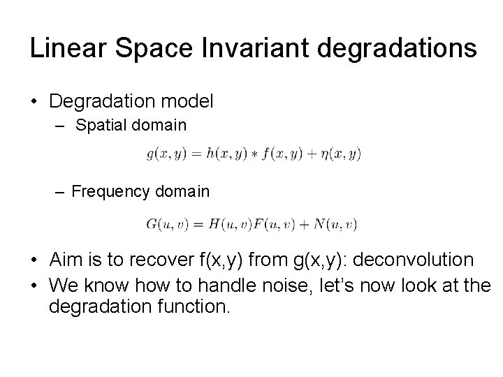
Linear Space Invariant degradations • Degradation model – Spatial domain – Frequency domain • Aim is to recover f(x, y) from g(x, y): deconvolution • We know how to handle noise, let’s now look at the degradation function.

Estimating the degradation function • 3 ways to estimate h(x, y) or H(u, v) – Observation • Observe certain areas in the image from which the degradation process is clear. – Experimentation • In case you have the equipment used to capture the degraded image – Mathematical modeling • If you know the degradation process, propose math models that will approximate the degradation.

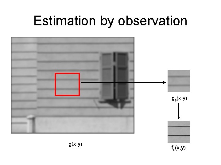
Estimation by observation • Degradation is assumed to be space invariant. • Look for part of image with simple structure – points, edges. • Since we know the ideal structure in this case, we can guess what was the original image.

Estimation by observation gs(x, y) g(x, y) fs(x, y)

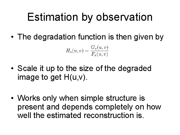
Estimation by observation • The degradation function is then given by • Scale it up to the size of the degraded image to get H(u, v). • Works only when simple structure is present and depends completely on how well the estimated reconstruction is.

Experimentation • If you have the imaging equipment causing the degradation, try getting images with different settings until they are similar to the given degraded image. • With the same settings compute the impulse response of the system by capturing an image of a light dot, which will give h(x, y). • The impulse response of a camera is called the Point Spread Function (PSF).

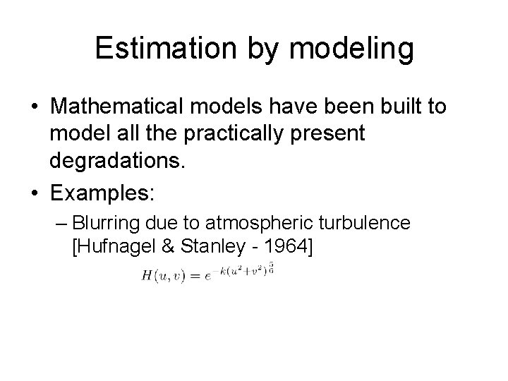
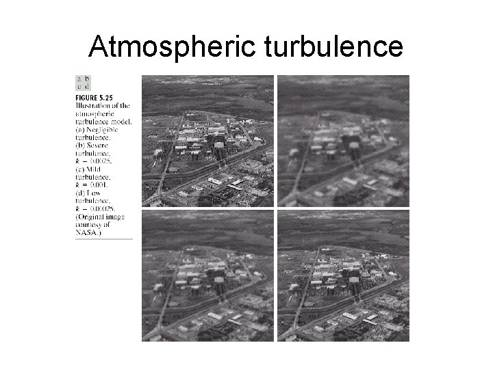
Estimation by modeling • Mathematical models have been built to model all the practically present degradations. • Examples: – Blurring due to atmospheric turbulence [Hufnagel & Stanley - 1964]

Atmospheric turbulence

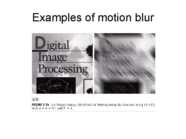
Motion blur • Blur due to motion of object relative to the imaging system. • Assume that the processes of opening and closing of shutter takes place instantaneously. • Assume that the imaging system is otherwise perfect. • Let ‘T’ be the time for which the shutter stays open

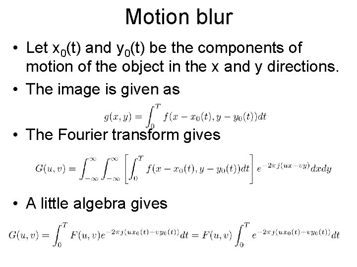
Motion blur • Let x 0(t) and y 0(t) be the components of motion of the object in the x and y directions. • The image is given as • The Fourier transform gives • A little algebra gives

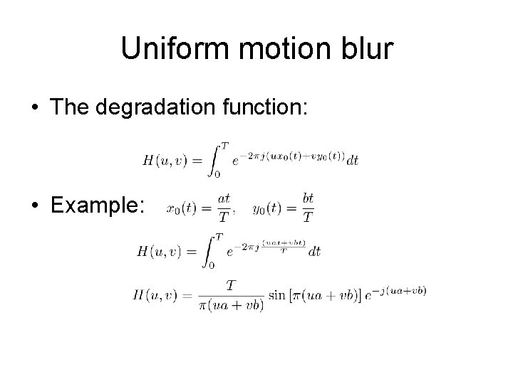
Uniform motion blur • The degradation function: • Example:

Examples of motion blur