Image Processing Lesson 10 Image Representation Gaussian pyramids

Image Processing - Lesson 10 Image Representation • Gaussian pyramids • Laplacian Pyramids • Wavelet Pyramids • Applications

Image Pyramids Image features at different resolutions require filters at different scales. Edges (derivatives): f(x) f (x)

Image Pyramids Image Pyramid = Hierarchical representation of an image Low Resolution No details in image (blurred image) low frequencies High Resolution Details in image low+high frequencies A collection of images at different resolutions.

Image pyramids • Gaussian Pyramids • Laplacian Pyramids • Wavelet/QMF

Image Pyramid Low resolution High resolution

Image Pyramid Frequency Domain Low resolution High resolution

Image Blurring = low pass filtering ~ = = *

Image Pyramid Low resolution High resolution

Gaussian Pyramid Level n 1 X 1 Level 1 2 n-1 X 2 n-1 Level 0 2 n X 2 n

Gaussian Pyramid

Gaussian Pyramid Burt & Adelson (1981) Normalized: Swi = 1 Symmetry: wi = w-i Unimodal: wi ³ wj for 0 < i < j Equal Contribution: for all j w-2 w 0 w 1 w-2 w-1 w 0 w 1 w 2 w-1 Swj+2 i = constant w 2

Gaussian Pyramid Burt & Adelson (1981) c b a b c c a + 2 b + 2 c = 1 a + 2 c = 2 b a > 0. 25 b = 0. 25 c = 0. 25 - a/2

For a = 0. 4 most similar to a Gauusian filter g = [0. 05 0. 25 0. 4 0. 25 0. 05] low_pass_filter = g’ * g = 0. 0025 0. 0125 0. 0200 0. 0125 0. 0025 0. 0125 0. 0625 0. 1000 0. 0625 0. 0125 0. 0200 0. 1000 0. 1600 0. 1000 0. 0200 0. 0125 0. 0625 0. 1000 0. 0625 0. 0125 0. 0025 0. 0125 0. 0200 0. 0125 0. 0025 0. 2 0. 15 0. 1 0. 05 0 5 4 3 3 2 2 1 1

Gaussian Pyramid Computational Aspects Memory: 2 NX 2 N (1 + 1/4 + 1/16 +. . . ) = 2 NX 2 N * 4/3 Computation: Level i can be computed with a single convolution with filter: hi = g * g *. . . i times Example: = * h 2 = g g

Multi. Scale Pattern Matching Option 1: Scale target and search for each in image. Option 2: Search for original target in image pyramid.

Hierarchical Pattern Matching search

Pattern matching using Pyramids - Example image pattern correlation

Image pyramids • Gaussian Pyramids • Laplacian Pyramids • Wavelet/QMF

Laplacian Pyramid Motivation = Compression, redundancy removal. compression rates are higher for predictable values. e. g. values around 0. G 0, G 1, . . = the levels of a Gaussian Pyramid. Predict level Gl from level Gl+1 by Expanding Gl+1 to G’l Gl+1 Expand Reduce Gl G’l Denote by Ll the error in prediction: Ll = Gl - G’l L 0, L 1, . . = the levels of a Laplacian Pyramid.

What does blurring take away? original

What does blurring take away? smoothed (5 x 5 Gaussian)

What does blurring take away? smoothed – original

Laplacian Pyramid Gaussian Pyramid expa n - d ex pa nd ex = - = pa nd

Gaussian Pyramid Frequency Domain Laplacian Pyramid

Laplace Pyramid No scaling

from: B. Freeman

Reconstruction of the original image from the Laplacian Pyramid Gl = Ll + G’l Laplacian Pyramid expand = + expand + = = Original Image

Laplacian Pyramid Computational Aspects Memory: 2 NX 2 N (1 + 1/4 + 1/16 +. . . ) = 2 NX 2 N * 4/3 However coefficients are highly compressible. Computation: Li can be computed from G 0 with a single convolution with filter: ki = hi-1 - hi - = hi-1 hi k 1 k 2 ki k 3

Image Mosaicing Registration

Image Blending

Blending

Multiresolution Spline When splining two images, transition from one image to the other should behave: High Frequencies Middle Frequencies Low Frequencies

Multiresolution Spline High Frequencies Middle Frequencies Low Frequencies

Multiresolution Spline - Example Left Image Right Image Left + Right Narrow Transition Wide Transition (Burt & Adelson)

Multiresolustion Spline - Using Laplacian Pyramid

Multiresolution Spline - Example Left Image Right Image Left + Right Narrow Transition Wide Transition Multiresolution Spline (Burt & Adelson)

Multiresolution Spline - Example Original - Left Original - Right Glued Splined

laplacian level 4 laplacian level 2 laplacian level 0 left pyramid right pyramid blended pyramid

Multiresolution Spline

Multiresolution Spline - Example

The colored version © prof. dmartin

Image pyramids • Gaussian Pyramids • Laplacian Pyramids • Wavelet/QMF

What is a good representation for image analysis? • Pixel domain representation tells you “where” (pixel location), but not “what”. – In space, this representation is too localized • Fourier transform domain tells you “what” (textural properties), but not “where”. – In space, this representation is too spread out. • Want an image representation that gives you a local description of image events —what is happening where. – That representation might be “just right”.

Space-Frequency Tiling Freq. Standard basis Spatial Freq. Fourier basis Spatial Freq. Wavelet basis Spatial

Space-Frequency Tiling Freq. Standard basis Spatial Freq. Fourier basis Spatial Freq. Wavelet basis Spatial

Various Wavelet basis

Wavelet - Frequency domain Wavelet bands are split recursively image H L L H H L

Wavelet - Frequency domain Wavelet decomposition - 2 D Frequency domain Horizontal high pass Vertical high pass Horizontal low pass Vertical low pass

Wavelet - Frequency domain Apply the wavelet transform separably in both dimensions Horizontal high pass, vertical high pass Horizontal low pass, vertical high-pass Horizontal high pass, vertical low-pass Horizontal low pass, Vertical low-pass

• Splitting can be applied recursively:

Pyramids in Frequency Domain Gaussian Pyramid Laplacian Pyramid

Wavelet Decomposition Fourier Space

Wavelet Transform - Step By Step Example

Wavelet Transform - Example

Wavelet Transform - Example

Image Pyramids - Comparison Image pyramid levels = Filter then sample. Filters: Gaussian Pyramid Laplacian Pyramid Wavelet Pyramid

Image Linear Transforms Transform Basis Characteristics Localized in space Not localized in Frequency Delta Standard Fourier Sines+Cosines Not localized in space Localized in Frequency Wavelet Pyramid Wavelet Filters Localized in space Localized in Frequency Delta space Fourier space Wavelet space

Convolution and Transforms in matrix notation (1 D case) transformed image Vectorized image Basis vectors (Fourier, Wavelet, etc)

Fourier Transform = Fourier transform * Fourier bases pixel domain image Fourier bases are global: each transform coefficient depends on all pixel locations. From: B. Freeman

Transform in matrix notation (1 D case) Forward Transform: transformed image Vectorized image Basis vectors (Fourier, Wavelet, etc) Inverse Transform: Basis vectors transformed image Vectorized image

Inverse Fourier Transform * Fourier bases = Fourier pixel domain transform image Every image pixel is a linear combination of the Fourier basis weighted by the coefficient. Note that if U is orthonormal basis then

Convolution = Convolution Result From: B. Freeman * Circular Matrix of Filter Kernels pixel image

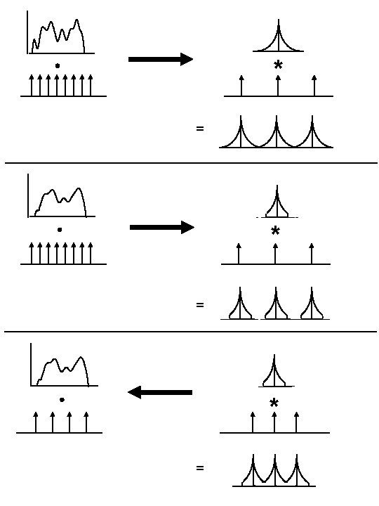
Pyramid = Convolution + Sampling = Convolution Result From: B. Freeman * Matrix of Filter Kernels pixel image

Pyramid = Convolution + Sampling Pyramid Level 1 = * Pyramid Level 2 = * *

Pyramid = Convolution + Sampling Pyramid Level 2 = * * Pyramid Level 2 = *

Pyramid as Matrix Computation - Example U 1 = 1 4 6 4 1 0 0 0 0 0 0 0 0 0 0 0 0 0 0 0 0 0 1 4 6 4 1 0 0 0 0 0 0 0 0 0 1 4 6 4 1 0 0 0 0 0 1 4 6 4 1 0 - Next pyramid level U 2 = 1 4 6 4 1 0 0 0 0 0 1 4 6 4 0 0 0 1 4 - The combined effect of the two pyramid levels U 2 * U 1 = 1 4 10 20 31 0 0 0 1 4 10 20 31 40 44 40 0 0 0 1 4 10 20 from: B. Freeman 40 44 40 31 20 40 10 44 4 40 1 0 0 0 20 10 4 1 0 0 0 30 16 4 0 25 16 4 0 31 0

Gaussian Pyramid = = * pixel image Gaussian pyramid Overcomplete representation. Low-pass filters, sampled appropriately for their blur. From: B. Freeman

Laplacian Pyramid = * pixel image Laplacian pyramid Overcomplete representation. Transformed pixels represent bandpassed image information. From: B. Freeman

Wavelet Transform = Wavelet pyramid * Ortho-normal transform (like Fourier transform), but with localized basis functions. From: B. Freeman pixel image

Wavelet Shrinkage Denoising

Image statistics (or, mathematically, how can you tell image from noise? ) Noisy image From: B. Freeman

Clean image From: B. Freeman

Image domain histogram From: B. Freeman

Wavelet domain image histogram From: B. Freeman

Image domain noise histogram From: B. Freeman

Wavelet domain noise histogram

Noise-corrupted full-freq and bandpass images But want the bandpass image histogram to look like this From: B. Freeman

Using Bayes theorem Constant w. r. t. parameters x. argmaxx P(x|y) = P(y|x) P(x) / P(y) The parameters you want to estimate Likelihood function What you observe Prior probability From: B. Freeman

Bayesian MAP estimator for clean bandpass coefficient values Let x = bandpassed image value before adding noise. Let y = noise-corrupted observation. By Bayes theorem P(x|y) = k P(y|x) P(x) maximum y P(y|x) P(x|y) From: B. Freeman

Bayesian MAP estimator for clean bandpass coefficient values y P(y|x) maximum P(x|y) From: B. Freeman

Bayesian MAP estimator for clean bandpass coefficient values y maximum P(y|x) P(x|y) From: B. Freeman

MAP estimate, , as function of observed coefficient value, y From: B. Freeman

Wavelet Shrinkage Pipe-line Mapping functions Transform W xiw yiw Inverse Transform WT

Noise removal results Simoncelli and Adelson, Noise Removal via Bayesian Wavelet Coring From: B. Freeman

More results

More results