Image Processing Intro 2 CS week 6 1

Image Processing Intro 2 CS – week 6 1

Image Processing • Many devices now have cameras on them • Lots of image data recorded for computers to process. • But how are images processed? • How are they encoded? • This week we explore some basic operations on images. • Some tasks are incredibly complex (face recognition, navigation by video, etc. ) 2

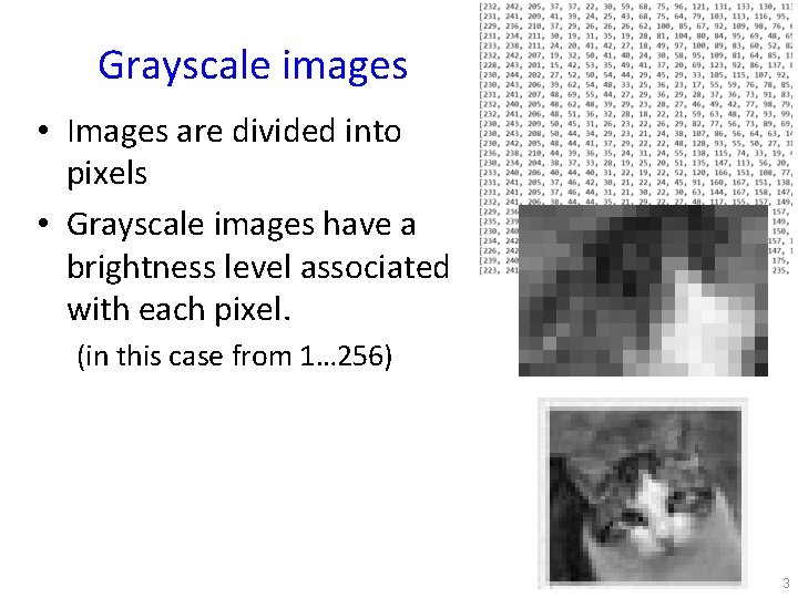
Grayscale images • Images are divided into pixels • Grayscale images have a brightness level associated with each pixel. (in this case from 1… 256) 3

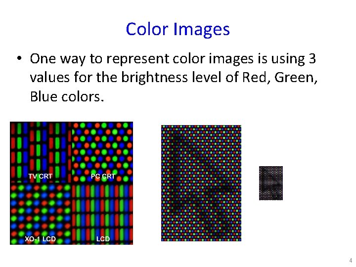
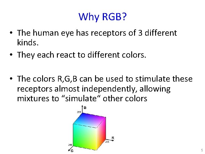
Color Images • One way to represent color images is using 3 values for the brightness level of Red, Green, Blue colors. 4

Why RGB? • The human eye has receptors of 3 different kinds. • They each react to different colors. • The colors R, G, B can be used to stimulate these receptors almost independently, allowing mixtures to “simulate“ other colors 5

Image Processing in Python • We will be using the Pillow library in python. • It can read images from files, show them (and do some processing – but we will do that ourselves). Find it here: • https: //pillow. readthedocs. org/ • I am using Win. Python (for windows) that comes pre-packaged with Pillow (and many other useful packages) http: //winpython. sourceforge. net/ • As usual, code show in this lecture, is available on the website. 6

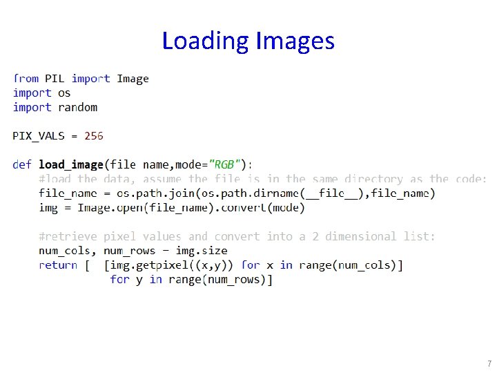
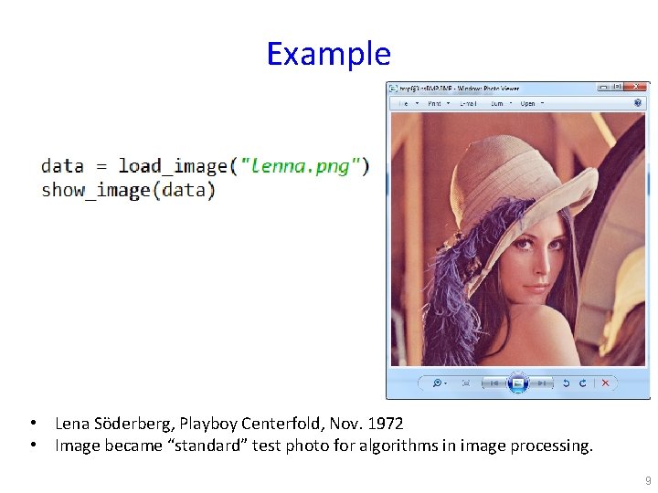
Loading Images 7

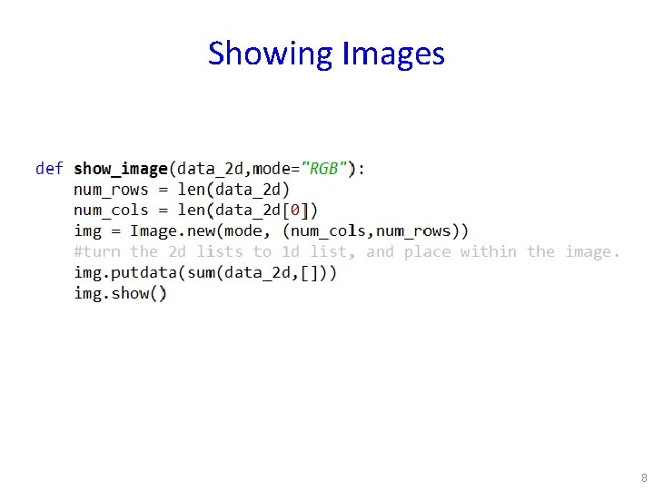
Showing Images 8

Example • Lena Söderberg, Playboy Centerfold, Nov. 1972 • Image became “standard” test photo for algorithms in image processing. 9

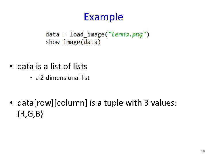
Example • data is a list of lists • a 2 -dimensional list • data[row][column] is a tuple with 3 values: (R, G, B) 10

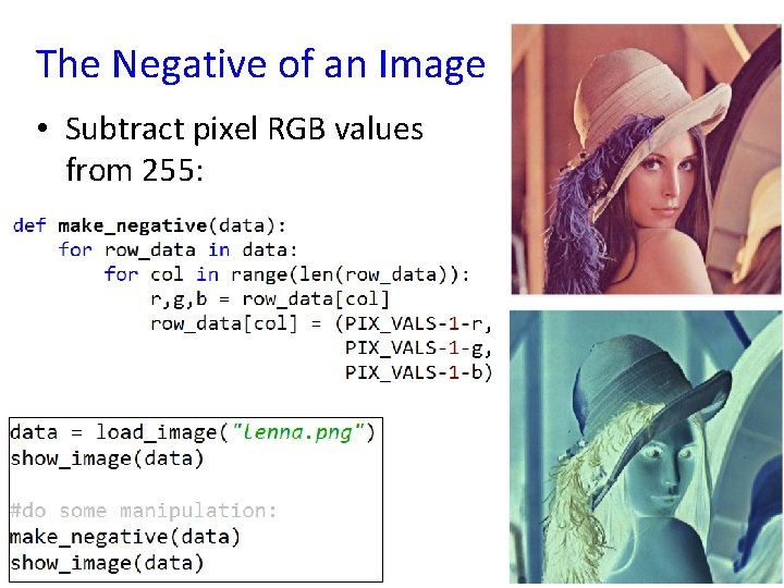
The Negative of an Image • Subtract pixel RGB values from 255: 11

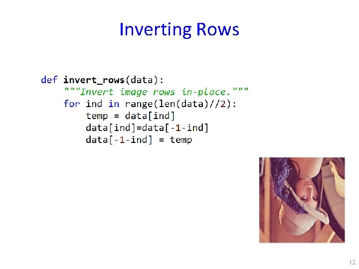
Inverting Rows 12

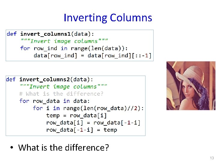
Inverting Columns • What is the difference? 13

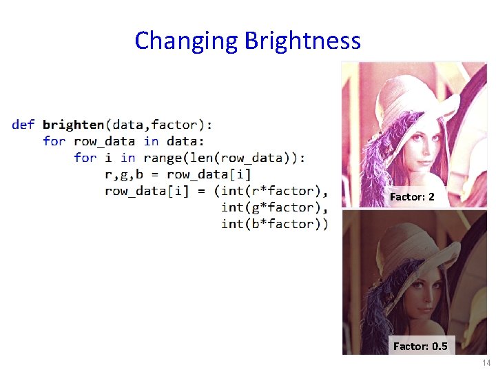
Changing Brightness Factor: 2 Factor: 0. 5 14

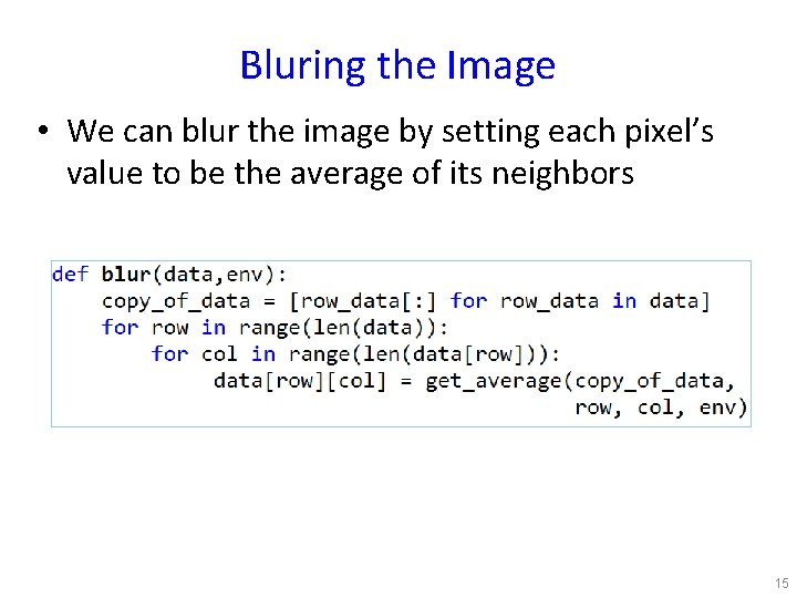
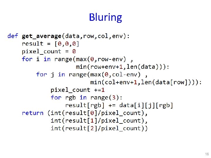
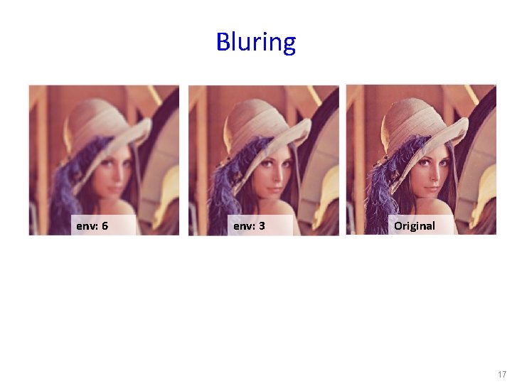
Bluring the Image • We can blur the image by setting each pixel’s value to be the average of its neighbors 15

Bluring 16

Bluring env: 6 env: 3 Original 17

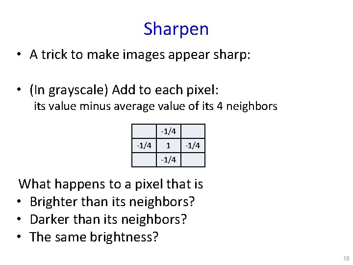
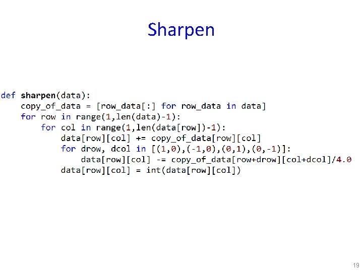
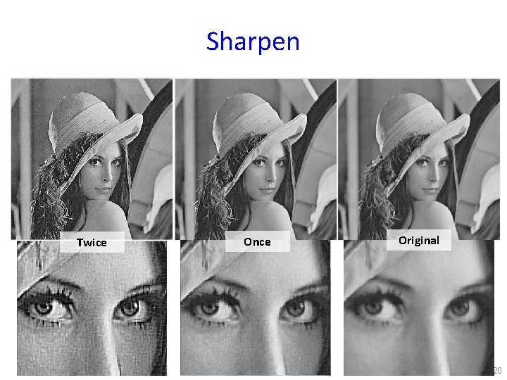
Sharpen • A trick to make images appear sharp: • (In grayscale) Add to each pixel: its value minus average value of its 4 neighbors -1/4 1 -1/4 What happens to a pixel that is • Brighter than its neighbors? • Darker than its neighbors? • The same brightness? 18

Sharpen 19

Sharpen Twice Once Original 20

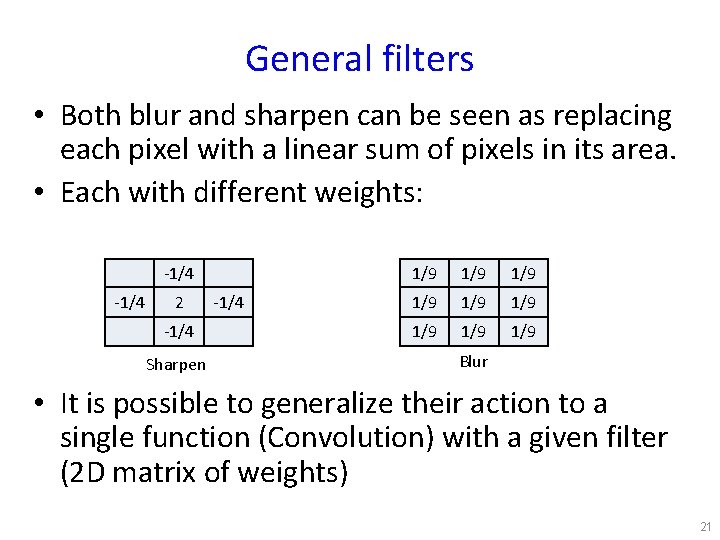
General filters • Both blur and sharpen can be seen as replacing each pixel with a linear sum of pixels in its area. • Each with different weights: -1/4 2 -1/4 Sharpen -1/4 1/9 1/9 1/9 Blur • It is possible to generalize their action to a single function (Convolution) with a given filter (2 D matrix of weights) 21

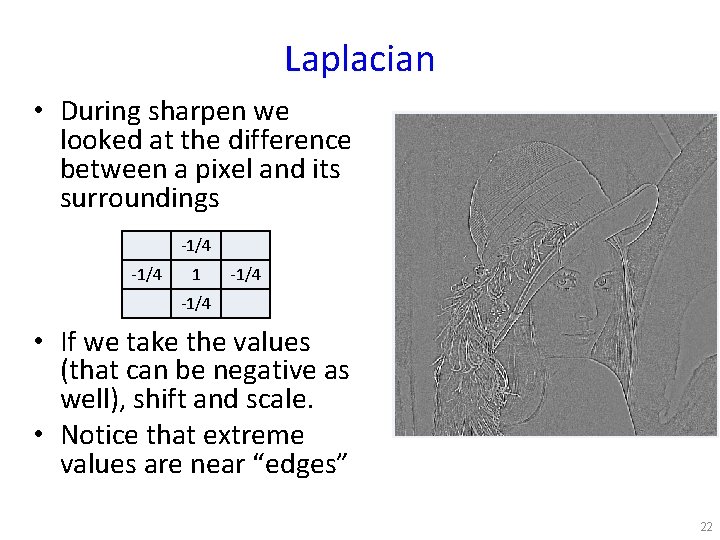
Laplacian • During sharpen we looked at the difference between a pixel and its surroundings -1/4 1 -1/4 • If we take the values (that can be negative as well), shift and scale. • Notice that extreme values are near “edges” 22

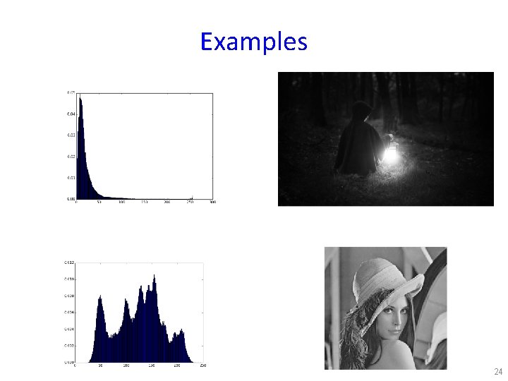
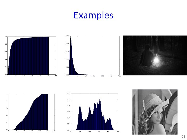
Histograms • We can look at statistics of pixel values in an image. • The histogram: for luminosity values 0. . . 255, how many pixels have each value? • Usually we’ll normalize: what is the percentage of pixels at each value 0. . . 255? 23

Examples 24

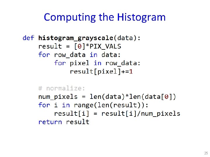
Computing the Histogram 25

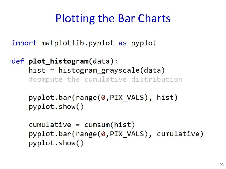
Plotting the Bar Charts 26

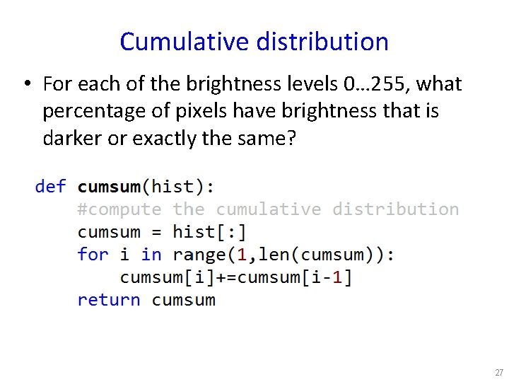
Cumulative distribution • For each of the brightness levels 0… 255, what percentage of pixels have brightness that is darker or exactly the same? 27

Examples 28

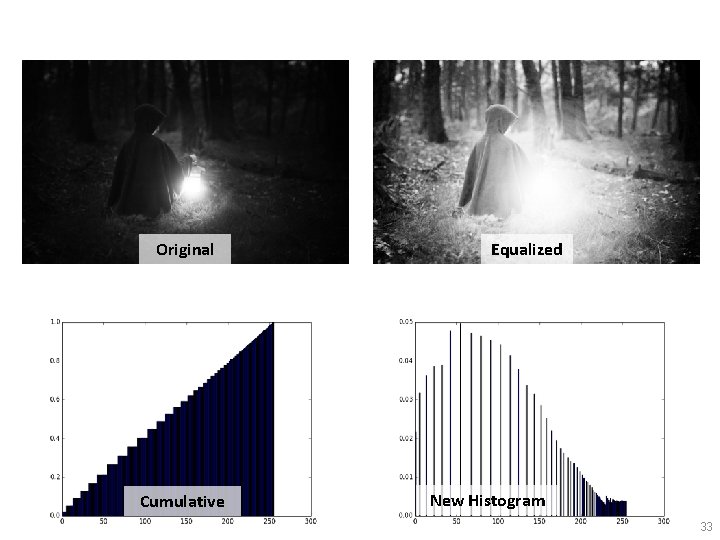
“Balanced” Histograms • An image that is properly exposed usually has pixels going all the way from dark to very bright. • The “ideal”: an equal amount of pixels for each brightness level • Can we shift the brightness levels so that this will happen? 29

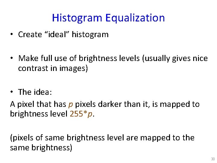
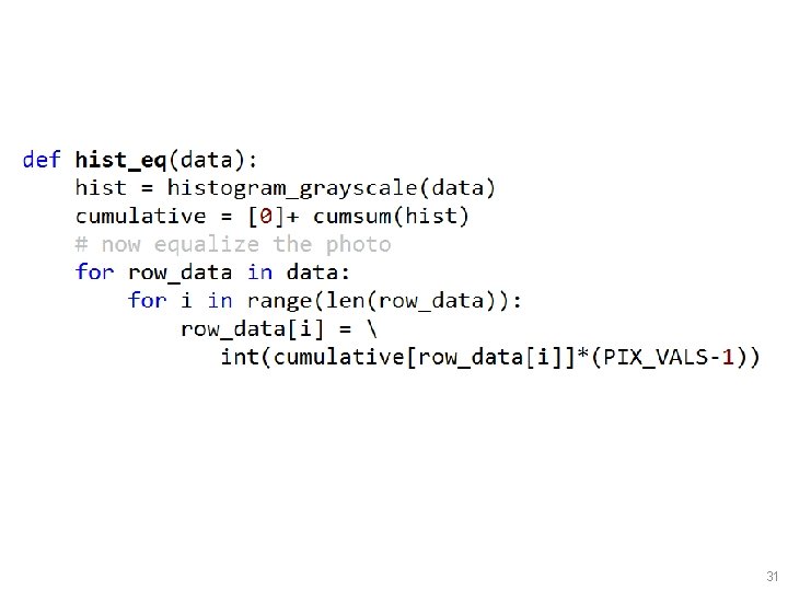
Histogram Equalization • Create “ideal” histogram • Make full use of brightness levels (usually gives nice contrast in images) • The idea: A pixel that has p pixels darker than it, is mapped to brightness level 255*p. (pixels of same brightness level are mapped to the same brightness) 30

31

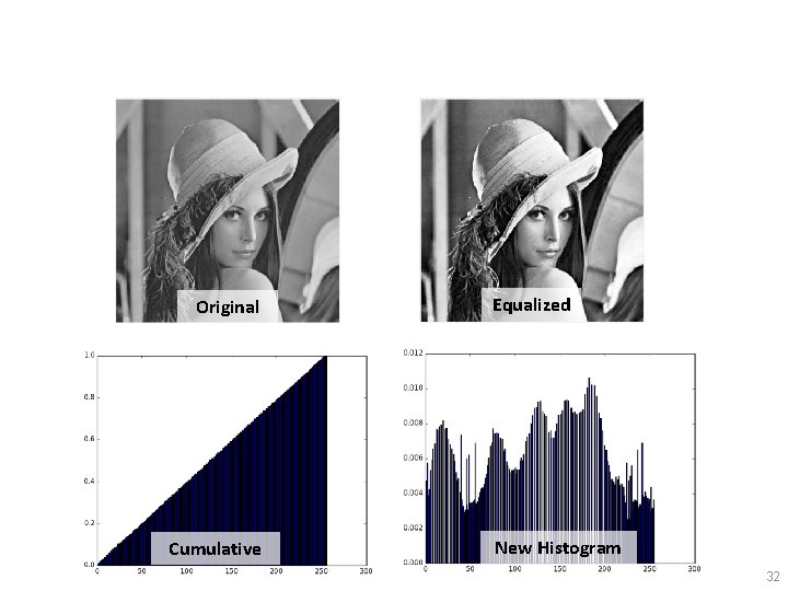
Original Cumulative Equalized New Histogram 32

Original Cumulative Equalized New Histogram 33

Extras 34

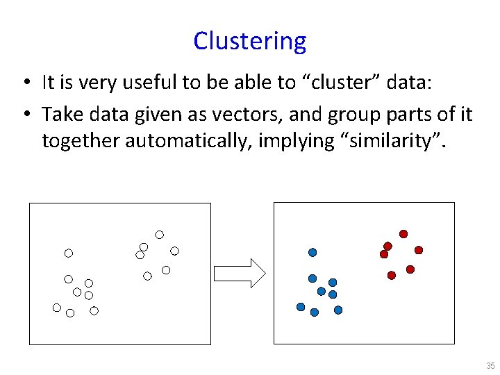
Clustering • It is very useful to be able to “cluster” data: • Take data given as vectors, and group parts of it together automatically, implying “similarity”. 35

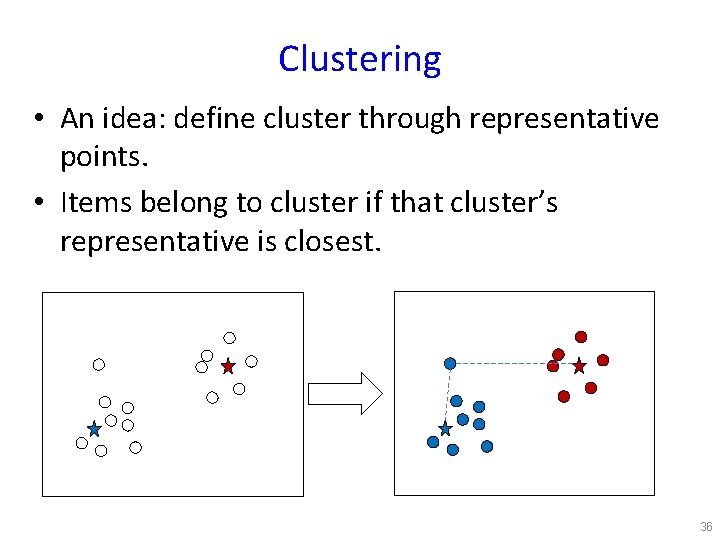
Clustering • An idea: define cluster through representative points. • Items belong to cluster if that cluster’s representative is closest. 36

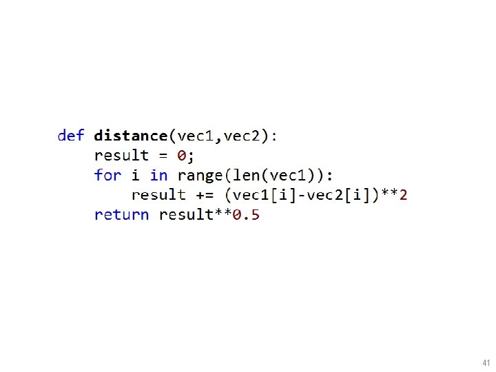
Clustering • What is a good partition to clusters? – Find cluster centers such that sum of distances of points to their cluster is minimized. • How do we solve this problem? 37

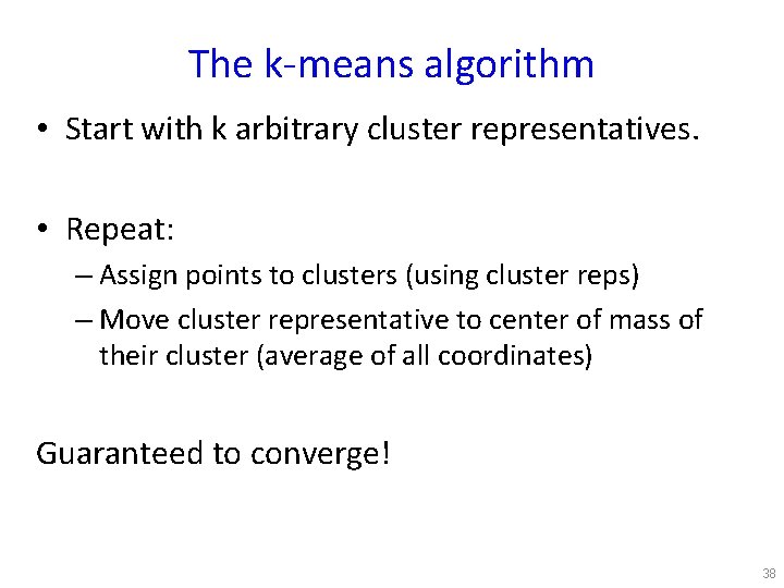
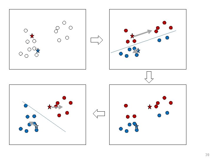
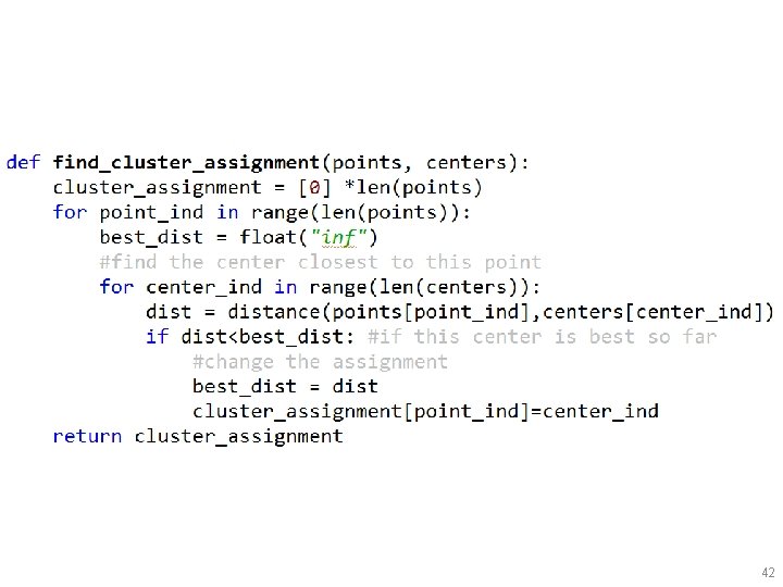
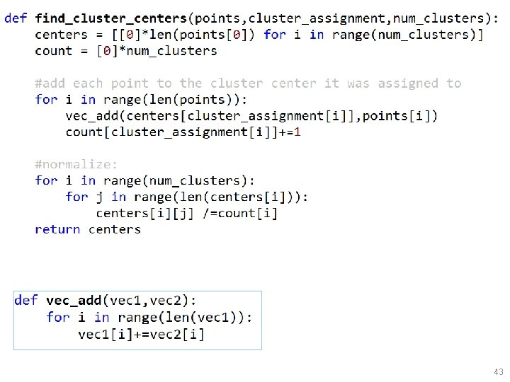
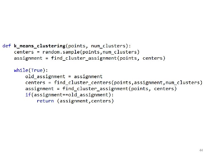
The k-means algorithm • Start with k arbitrary cluster representatives. • Repeat: – Assign points to clusters (using cluster reps) – Move cluster representative to center of mass of their cluster (average of all coordinates) Guaranteed to converge! 38

39

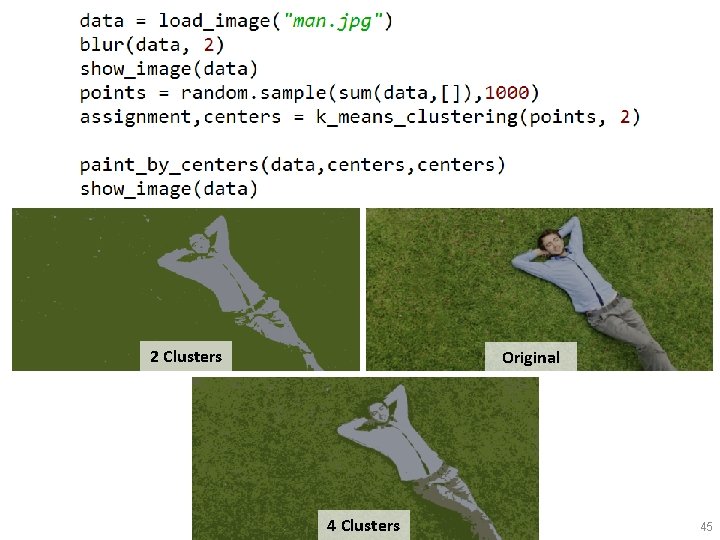
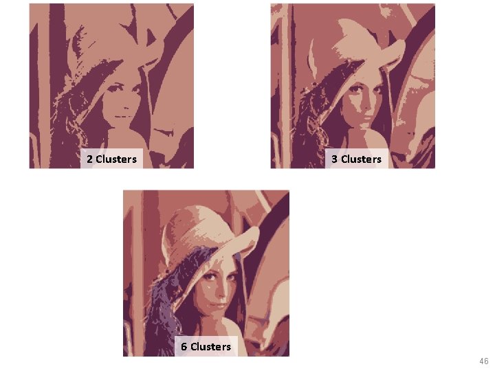
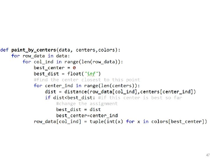
Applying to images • We’ll apply k-means to images. • Find clusters of pixel colors • Use them to segment the image into pixels that contain “similar things” (as we can judge by color). 40

41

42

43

44

2 Clusters Original 4 Clusters 45

2 Clusters 3 Clusters 6 Clusters 46

47