Image Processing Index Geometric enhancement low pass filters

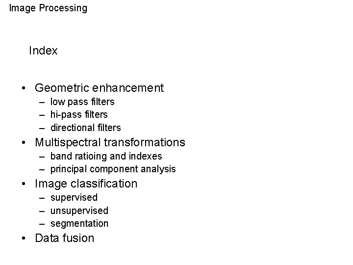
Image Processing Index • Geometric enhancement – low pass filters – hi-pass filters – directional filters • Multispectral transformations – band ratioing and indexes – principal component analysis • Image classification – supervised – unsupervised – segmentation • Data fusion

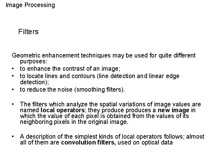
Image Processing Filters Geometric enhancement techniques may be used for quite different purposes: • to enhance the contrast of an image; • to locate lines and contours (line detection and linear edge detection); • to reduce the noise (smoothing filters). • The filters which analyze the spatial variations of image values are named local operators; they produces a new image in which the value of each pixel is obtained from the values of its neighboring pixels in the original image. • A description of the simplest kinds of local operators follows; almost all of them are convolution filters, used on optical data

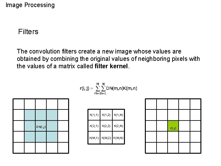
Image Processing Filters The convolution filters create a new image whose values are obtained by combining the original values of neighboring pixels with the values of a matrix called filter kernel. DN(i, j) K(1, 1) K(1, 2) K(1, N) K(2, 1) K(2, 2) K(2, N) K(M, 1) K(M, 2) K(M, N) r(i, j)

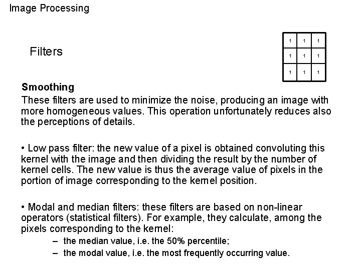
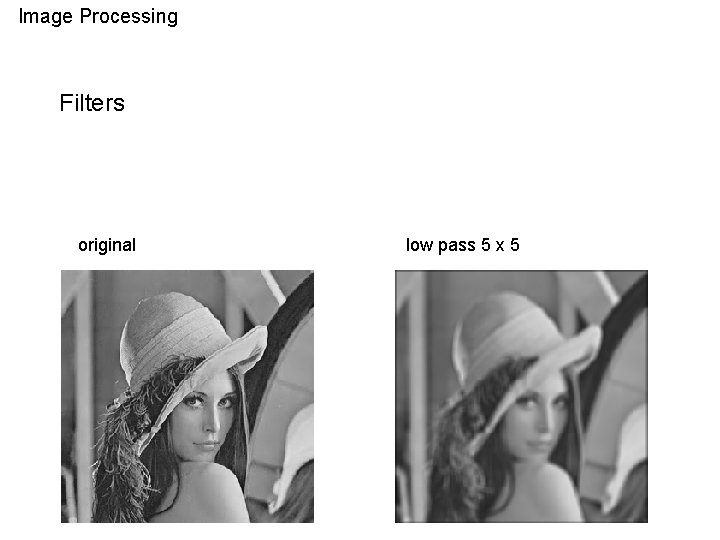
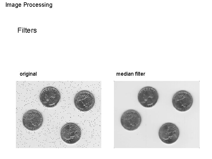
Image Processing Filters 1 1 1 1 1 Smoothing These filters are used to minimize the noise, producing an image with more homogeneous values. This operation unfortunately reduces also the perceptions of details. • Low pass filter: the new value of a pixel is obtained convoluting this kernel with the image and then dividing the result by the number of kernel cells. The new value is thus the average value of pixels in the portion of image corresponding to the kernel position. • Modal and median filters: these filters are based on non-linear operators (statistical filters). For example, they calculate, among the pixels corresponding to the kernel: – the median value, i. e. the 50% percentile; – the modal value, i. e. the most frequently occurring value.

Image Processing Filters original low pass 5 x 5

Image Processing Filters original median filter

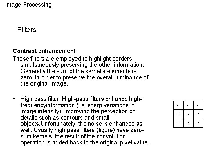
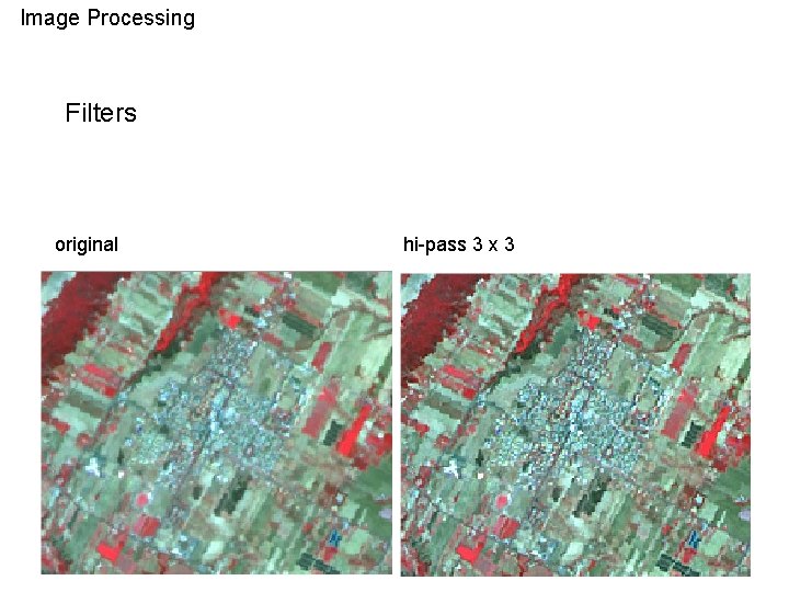
Image Processing Filters Contrast enhancement These filters are employed to highlight borders, simultaneously preserving the other information. Generally the sum of the kernel’s elements is zero, in order to preserve the overall luminance of the original image. • High pass filter: High-pass filters enhance highfrequencyinformation (i. e. sharp variations in image intensity), improving the perception of details such as contours and small objects. Unfortunately, the noise is enhanced as well. Usually high pass filters (figure) have zerosum kernels: the result of the convolution operation is added back to the original pixel value. -1 -1 8 -1 -1

Image Processing Filters original hi-pass 3 x 3

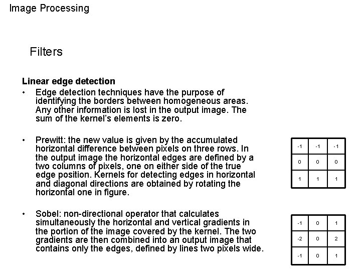
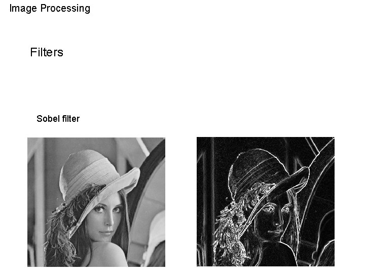
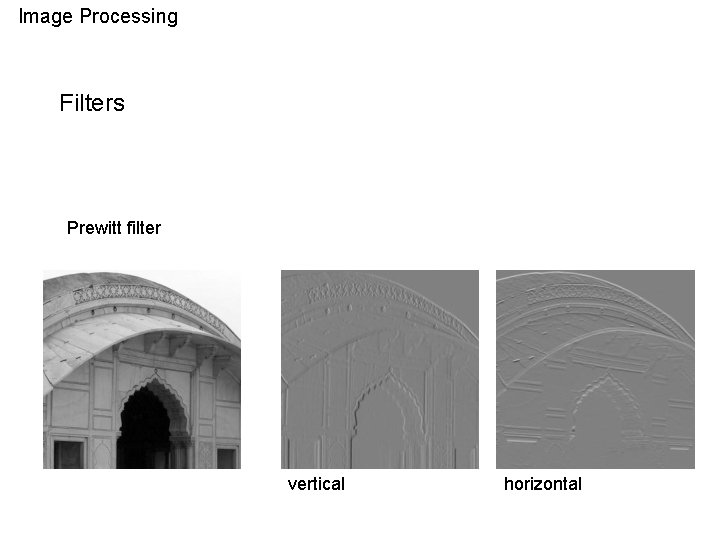
Image Processing Filters Linear edge detection • Edge detection techniques have the purpose of identifying the borders between homogeneous areas. Any other information is lost in the output image. The sum of the kernel’s elements is zero. • • Prewitt: the new value is given by the accumulated horizontal difference between pixels on three rows. In the output image the horizontal edges are defined by a two columns of pixels, one on either side of the true edge position. Kernels for detecting edges in horizontal and diagonal directions are obtained by rotating the horizontal one in figure. Sobel: non-directional operator that calculates simultaneously the horizontal and vertical gradients in the portion of the image covered by the kernel. The two gradients are then combined into an output image that contains only the edges, defined by lines two pixels wide. -1 -1 -1 0 0 0 1 1 1 -1 0 1 -2 0 2 -1 0 1

Image Processing Filters Sobel filter

Image Processing Filters Prewitt filter vertical horizontal

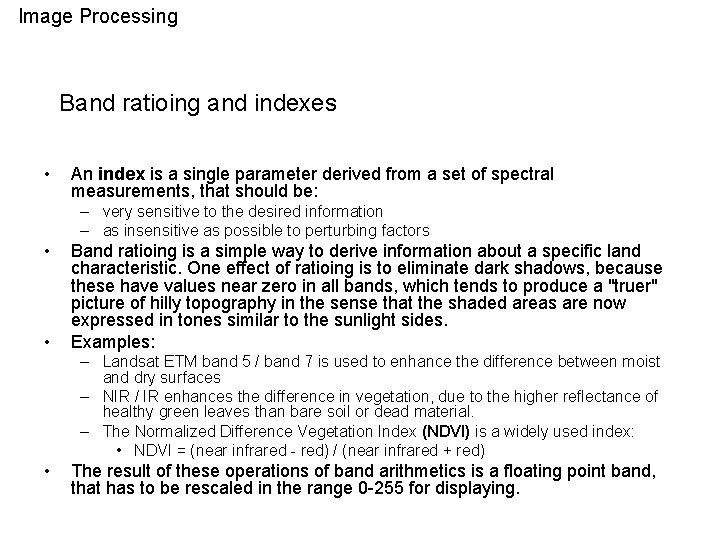
Image Processing Band ratioing and indexes • An index is a single parameter derived from a set of spectral measurements, that should be: – very sensitive to the desired information – as insensitive as possible to perturbing factors • • Band ratioing is a simple way to derive information about a specific land characteristic. One effect of ratioing is to eliminate dark shadows, because these have values near zero in all bands, which tends to produce a "truer" picture of hilly topography in the sense that the shaded areas are now expressed in tones similar to the sunlight sides. Examples: – Landsat ETM band 5 / band 7 is used to enhance the difference between moist and dry surfaces – NIR / IR enhances the difference in vegetation, due to the higher reflectance of healthy green leaves than bare soil or dead material. – The Normalized Difference Vegetation Index (NDVI) is a widely used index: • NDVI = (near infrared - red) / (near infrared + red) • The result of these operations of band arithmetics is a floating point band, that has to be rescaled in the range 0 -255 for displaying.

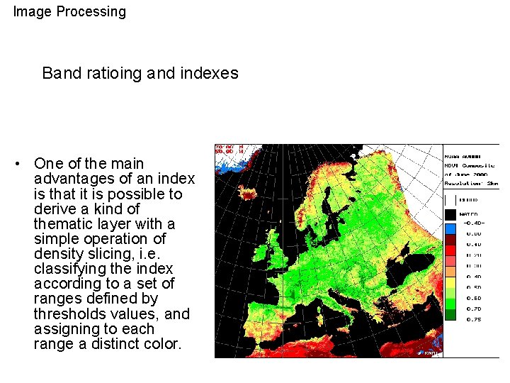
Image Processing Band ratioing and indexes • One of the main advantages of an index is that it is possible to derive a kind of thematic layer with a simple operation of density slicing, i. e. classifying the index according to a set of ranges defined by thresholds values, and assigning to each range a distinct color.

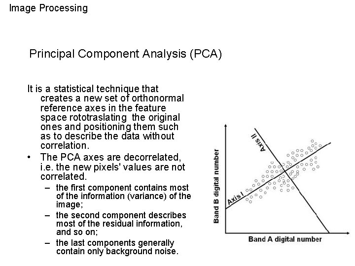
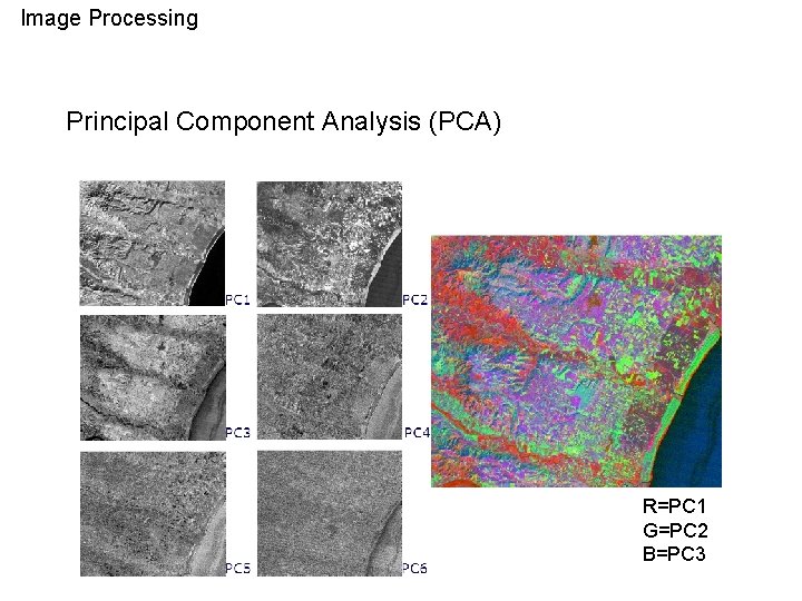
Image Processing Principal Component Analysis (PCA) It is a statistical technique that creates a new set of orthonormal reference axes in the feature space rototraslating the original ones and positioning them such as to describe the data without correlation. • The PCA axes are decorrelated, i. e. the new pixels' values are not correlated. – the first component contains most of the information (variance) of the image; – the second component describes most of the residual information, and so on; – the last components generally contain only background noise.

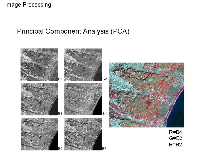
Image Processing Principal Component Analysis (PCA) R=B 4 G=B 3 B=B 2

Image Processing Principal Component Analysis (PCA) R=PC 1 G=PC 2 B=PC 3

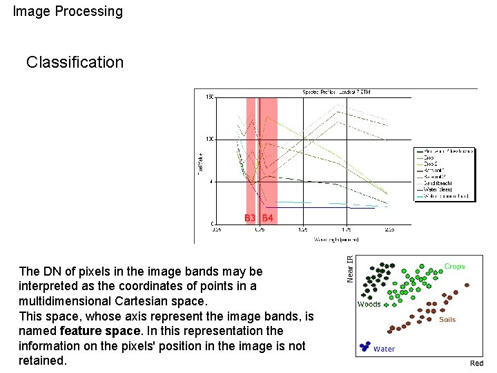
Image Processing Classification The DN of pixels in the image bands may be interpreted as the coordinates of points in a multidimensional Cartesian space. This space, whose axis represent the image bands, is named feature space. In this representation the information on the pixels' position in the image is not retained.

Image Processing Classification A pixel is classified by the assignment to a cluster corresponding to a type of surface, on the base of its position in the feature space. Problems: • Image pixels are often mixed, i. e. their surface is covered by more than one class of land cover. The point corresponding to a mixed pixel is located in the feature space somewhat between the groups of points representing the classes in the mix, and its assignment is therefore difficult. • Evaluation of the surfaces that may be effectively identified in the image. The clusters in the feature space identify surfaces characterized by different reflectance properties; these surfaces may differ from the ones that the user is interested in, for example: – water bodies characterized by high differences in suspended materials form separate groups in the feature space; this distinction may not be required in land cover maps; – the discrimination between two kinds of crops may be requested, but if the two crops have similar reflectance properties, it is impossible to distinguish them.

Image Processing Classification Supervised classification • It is commonly used to produce land cover maps from remote sensing imagery. • It is based on the use of ground truth data to identify the typical pixels' values of the land cover classes present in the image. This is equivalent to define the regions of the feature space that contain the points belonging to the classes that must be recognized in the image (“spectral signature”). • The pixels are assigned to a class by means of a comparison between their digital values and the typical digital values of the various land cover classes. This is equivalent to the analysis of the pixels' distance from the region of the feature space corresponding to the land cover classes. – – – Definition of a legend Collection of training set Definition of classes Classification Accuracy assessment

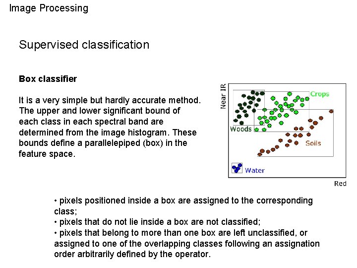
Image Processing Supervised classification Box classifier It is a very simple but hardly accurate method. The upper and lower significant bound of each class in each spectral band are determined from the image histogram. These bounds define a parallelepiped (box) in the feature space. • pixels positioned inside a box are assigned to the corresponding class; • pixels that do not lie inside a box are not classified; • pixels that belong to more than one box are left unclassified, or assigned to one of the overlapping classes following an assignation order arbitrarily defined by the operator.

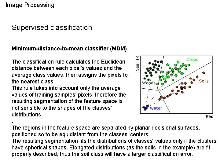
Image Processing Supervised classification Minimum-distance-to-mean classifier (MDM) The classification rule calculates the Euclidean distance between each pixel’s values and the average class values, then assigns the pixels to the nearest class This rule takes into account only the average values of training samples’ pixels; therefore the resulting segmentation of the feature space is not sensible to the shapes of the classes’ distributions. The regions in the feature space are separated by planar decisional surfaces, positioned so to be equidistant from the classes’ centers. The resulting segmentation fits the distributions of classes' values only if the clusters have spherical shapes. Elongated distributions (as the soils in the example) aren't properly described; thus the soil class will have a larger classification error.

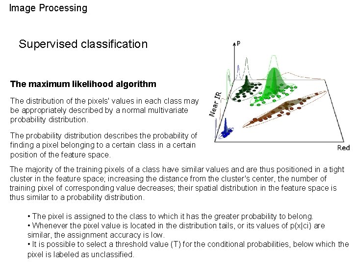
Image Processing Supervised classification The maximum likelihood algorithm The distribution of the pixels' values in each class may be appropriately described by a normal multivariate probability distribution. The probability distribution describes the probability of finding a pixel belonging to a certain class in a certain position of the feature space. The majority of the training pixels of a class have similar values and are thus positioned in a tight cluster in the feature space; increasing the distance from the cluster's center, the number of training pixel of corresponding value decreases; their spatial distribution in the feature space is thus similar to a probability distribution. • The pixel is assigned to the class to which it has the greater probability to belong. • Whenever the pixel value is located in the distribution tails, or its values of p(x|ci) are similar, the assignment accuracy is low. • It is possible to select a threshold value (T) for the conditional probabilities, below which the pixel is labeled as unclassified.

Image Processing Supervised classification The training stage is executed by an operator. Its quality is extremely important: it determines the quality of the final result. Two main goals: • define which classes can be identified in the image, • obtain the statistical parameters that describe the distribution of digital values in each class. Very important: completeness of samples. They must be acquired for all the kinds of reflective surfaces present in the imaged area. • the segmentation of the area into "reflective surfaces" is generally different from the surfaces that the user needs to identify in the image. – a land cover class is made up of pixels with great differences in spectral reflectivity (e. g. urban areas), so that the frequency distribution of reflectance values shows more than one peak, violating the basic hypothesis of the classification procedure. To perform the classification it is necessary to divide this multimodal class in several subclasses, each one characterized by unimodal distribution of DNs. The subclasse will be merged after the classification. – the reflectivity distributions of two or more land cover classes are too similar to be distinguishable with a low assignation error. It is a common case for agricultural croplands. In this case it is compulsory to merge the classes.

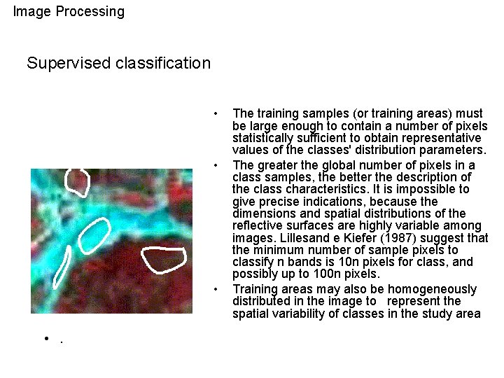
Image Processing Supervised classification • • . The training samples (or training areas) must be large enough to contain a number of pixels statistically sufficient to obtain representative values of the classes' distribution parameters. The greater the global number of pixels in a class samples, the better the description of the class characteristics. It is impossible to give precise indications, because the dimensions and spatial distributions of the reflective surfaces are highly variable among images. Lillesand e Kiefer (1987) suggest that the minimum number of sample pixels to classify n bands is 10 n pixels for class, and possibly up to 100 n pixels. Training areas may also be homogeneously distributed in the image to represent the spatial variability of classes in the study area

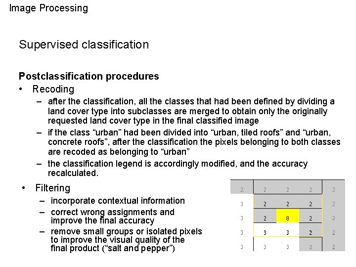
Image Processing Supervised classification Postclassification procedures • Recoding – after the classification, all the classes that had been defined by dividing a land cover type into subclasses are merged to obtain only the originally requested land cover type in the final classified image – if the class “urban” had been divided into “urban, tiled roofs” and “urban, concrete roofs”, after the classification the pixels belonging to both classes are recoded as belonging to “urban” – the classification legend is accordingly modified, and the accuracy recalculated. • Filtering – incorporate contextual information – correct wrong assignments and improve the final accuracy – remove small groups or isolated pixels to improve the visual quality of the final product (“salt and pepper”)

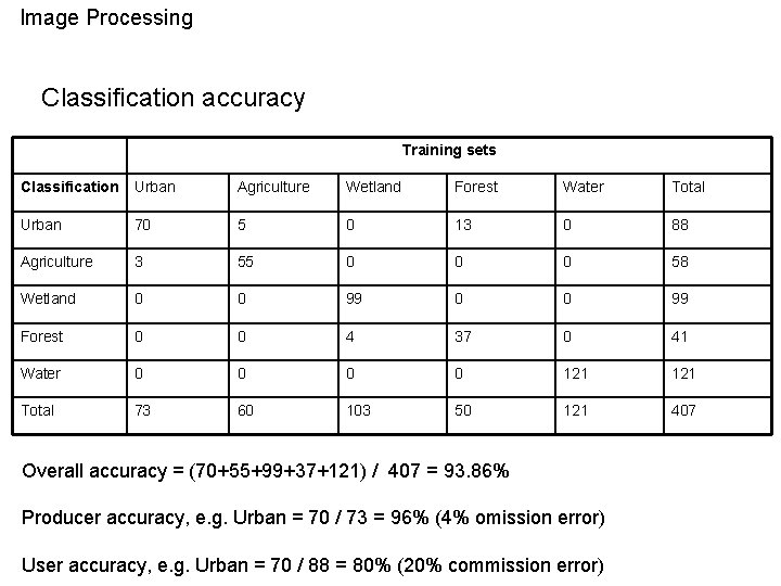
Image Processing Classification accuracy Training sets Classification Urban Agriculture Wetland Forest Water Total Urban 70 5 0 13 0 88 Agriculture 3 55 0 0 0 58 Wetland 0 0 99 Forest 0 0 4 37 0 41 Water 0 0 121 Total 73 60 103 50 121 407 Overall accuracy = (70+55+99+37+121) / 407 = 93. 86% Producer accuracy, e. g. Urban = 70 / 73 = 96% (4% omission error) User accuracy, e. g. Urban = 70 / 88 = 80% (20% commission error)

Image Processing Classification Unsupervised classification • No or little intervention of operator • It produces a more or less objective “inventory” of the different spectral objects present in the images • The feature space of the image is “seeded” with a certain number of randomly located points, that are used as cluster centroids. The pixels are then assigned to these clusters according to their distance from the first centroids. • The operation is repeated n times, and at each pass the clusters are statistically evaluated. Large clusters are splitted, small clusters ar merged, and new centroids are generated. • The iterations stop when the distance between centroids in two consecutive passes is smaller than an user-defined threshold. • Useful to get a quick-and-dirty knowledge about the spectral characteristic of the study area; it cannot replace a supervised approach.

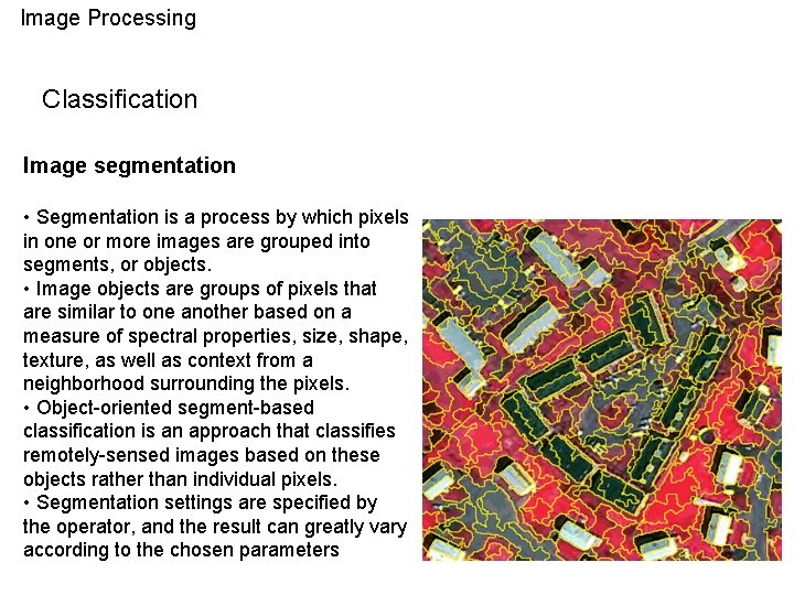
Image Processing Classification Image segmentation • Segmentation is a process by which pixels in one or more images are grouped into segments, or objects. • Image objects are groups of pixels that are similar to one another based on a measure of spectral properties, size, shape, texture, as well as context from a neighborhood surrounding the pixels. • Object-oriented segment-based classification is an approach that classifies remotely-sensed images based on these objects rather than individual pixels. • Segmentation settings are specified by the operator, and the result can greatly vary according to the chosen parameters

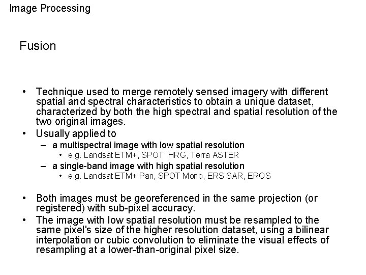
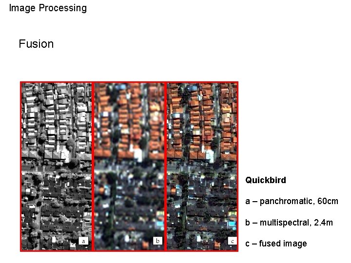
Image Processing Fusion • Technique used to merge remotely sensed imagery with different spatial and spectral characteristics to obtain a unique dataset, characterized by both the high spectral and spatial resolution of the two original images. • Usually applied to – a multispectral image with low spatial resolution • e. g. Landsat ETM+, SPOT HRG, Terra ASTER – a single-band image with high spatial resolution • e. g. Landsat ETM+ Pan, SPOT Mono, ERS SAR, EROS • Both images must be georeferenced in the same projection (or registered) with sub-pixel accuracy. • The image with low spatial resolution must be resampled to the same pixel's size of the higher resolution dataset, using a bilinear interpolation or cubic convolution to eliminate the visual effects of resampling at a lower-than-original pixel size.

Image Processing Fusion Quickbird a – panchromatic, 60 cm b – multispectral, 2. 4 m c – fused image

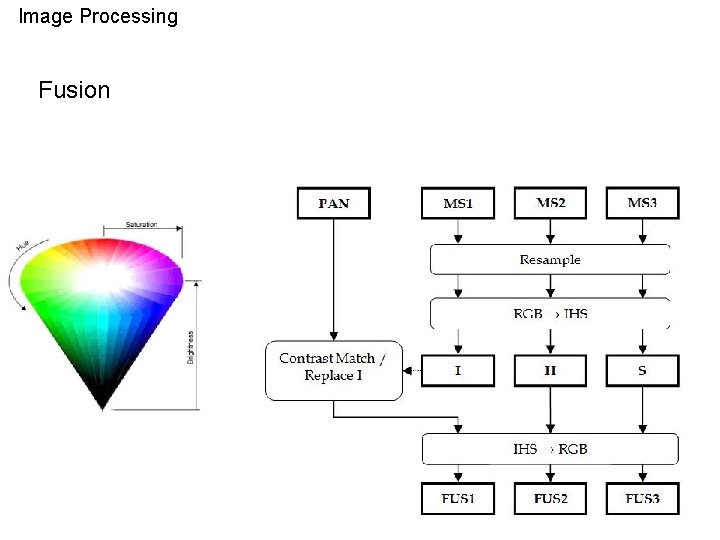
Image Processing Fusion

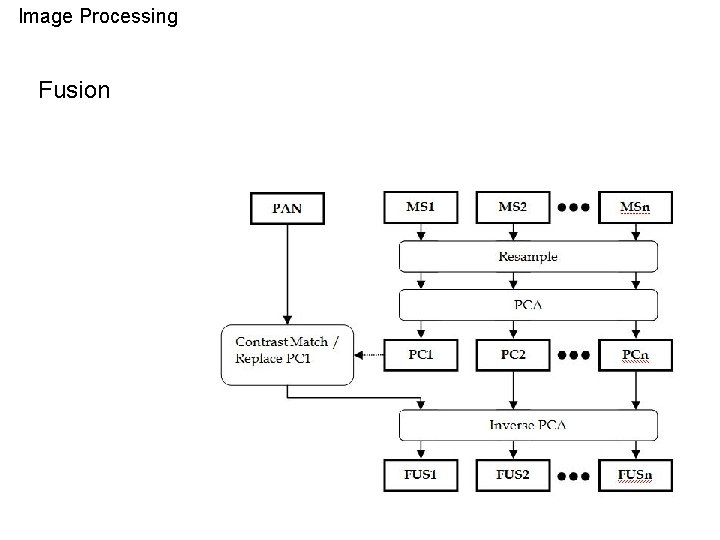
Image Processing Fusion