Image Processing Face Recognition Using Principal Components Analysis

Image Processing Face Recognition Using Principal Components Analysis (PCA) M. Turk, A. Pentland, "Eigenfaces for Recognition", Journal of Cognitive Neuroscience, 3(1), pp. 71 -86, 1991.

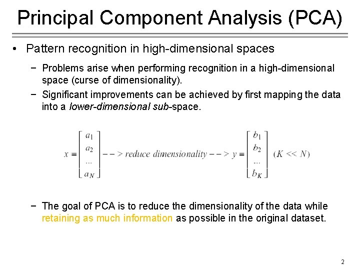
Principal Component Analysis (PCA) • Pattern recognition in high-dimensional spaces − Problems arise when performing recognition in a high-dimensional space (curse of dimensionality). − Significant improvements can be achieved by first mapping the data into a lower-dimensional sub-space. − The goal of PCA is to reduce the dimensionality of the data while retaining as much information as possible in the original dataset. 2

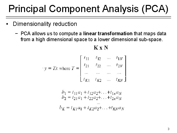
Principal Component Analysis (PCA) • Dimensionality reduction − PCA allows us to compute a linear transformation that maps data from a high dimensional space to a lower dimensional sub-space. K x N 3

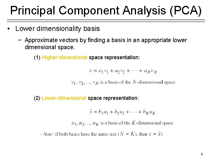
Principal Component Analysis (PCA) • Lower dimensionality basis − Approximate vectors by finding a basis in an appropriate lower dimensional space. (1) Higher-dimensional space representation: (2) Lower-dimensional space representation: 4

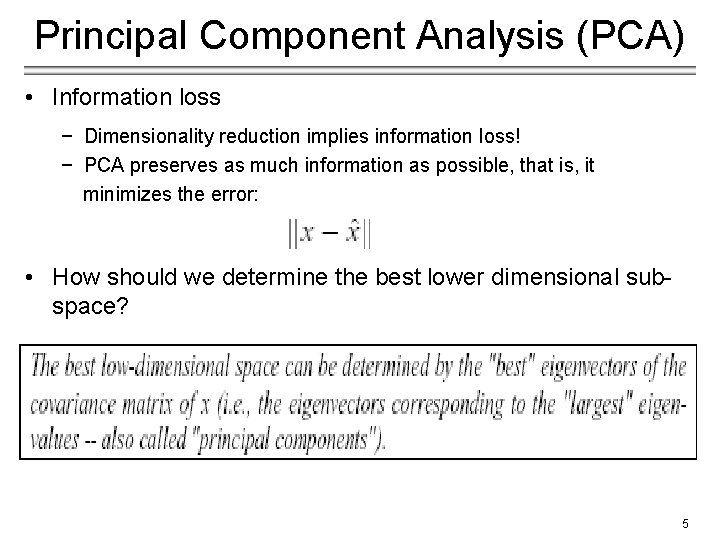
Principal Component Analysis (PCA) • Information loss − Dimensionality reduction implies information loss! − PCA preserves as much information as possible, that is, it minimizes the error: • How should we determine the best lower dimensional subspace? 5

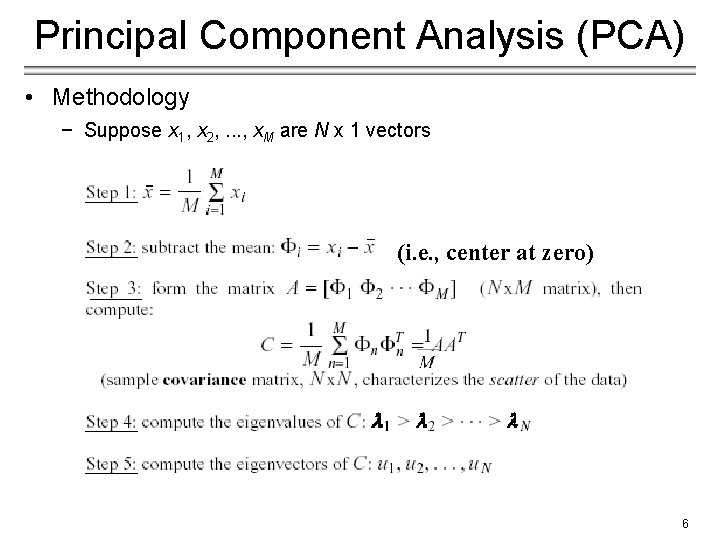
Principal Component Analysis (PCA) • Methodology − Suppose x 1, x 2, . . . , x. M are N x 1 vectors (i. e. , center at zero) 6

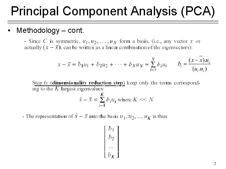
Principal Component Analysis (PCA) • Methodology – cont. 7

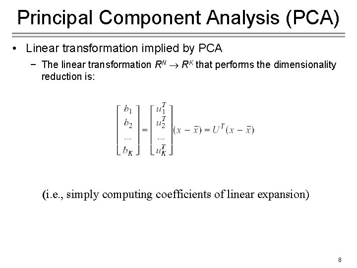
Principal Component Analysis (PCA) • Linear transformation implied by PCA − The linear transformation RN RK that performs the dimensionality reduction is: (i. e. , simply computing coefficients of linear expansion) 8

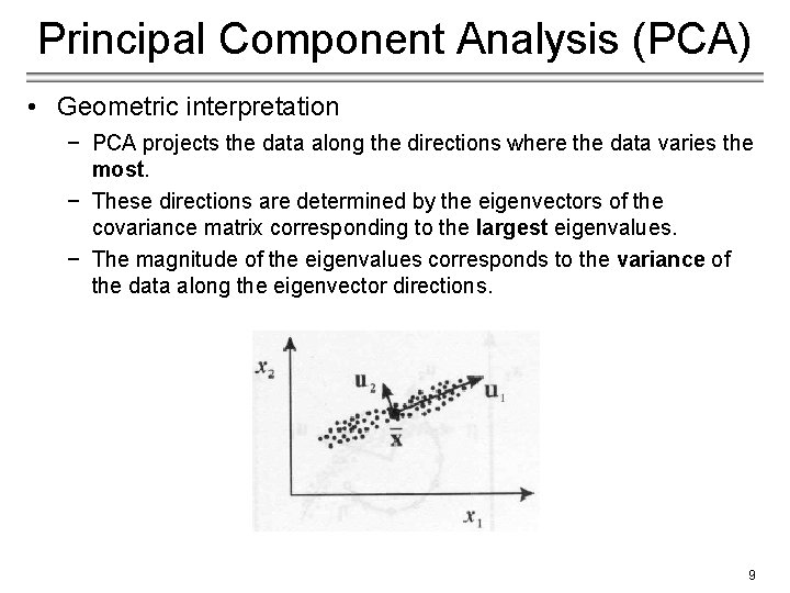
Principal Component Analysis (PCA) • Geometric interpretation − PCA projects the data along the directions where the data varies the most. − These directions are determined by the eigenvectors of the covariance matrix corresponding to the largest eigenvalues. − The magnitude of the eigenvalues corresponds to the variance of the data along the eigenvector directions. 9

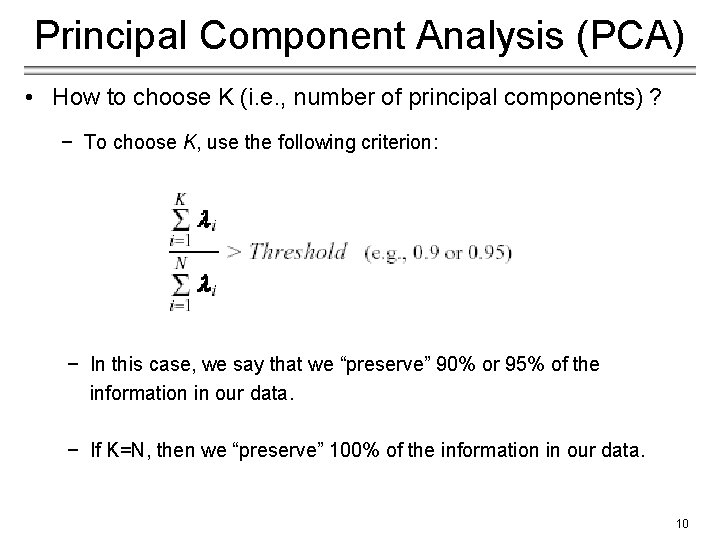
Principal Component Analysis (PCA) • How to choose K (i. e. , number of principal components) ? − To choose K, use the following criterion: − In this case, we say that we “preserve” 90% or 95% of the information in our data. − If K=N, then we “preserve” 100% of the information in our data. 10

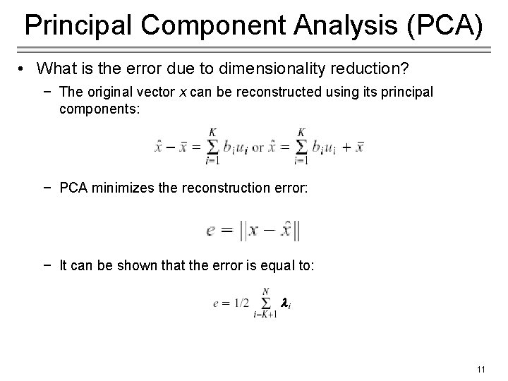
Principal Component Analysis (PCA) • What is the error due to dimensionality reduction? − The original vector x can be reconstructed using its principal components: − PCA minimizes the reconstruction error: − It can be shown that the error is equal to: 11

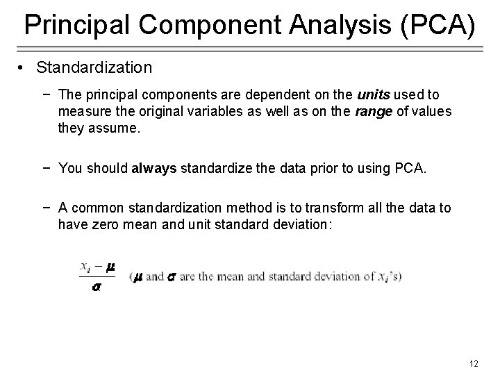
Principal Component Analysis (PCA) • Standardization − The principal components are dependent on the units used to measure the original variables as well as on the range of values they assume. − You should always standardize the data prior to using PCA. − A common standardization method is to transform all the data to have zero mean and unit standard deviation: 12

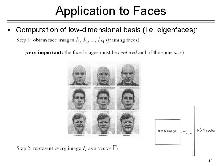
Application to Faces • Computation of low-dimensional basis (i. e. , eigenfaces): 13

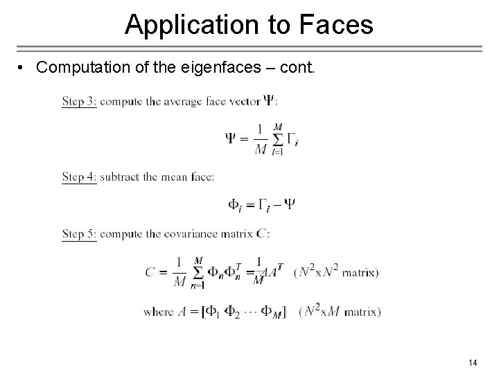
Application to Faces • Computation of the eigenfaces – cont. 14

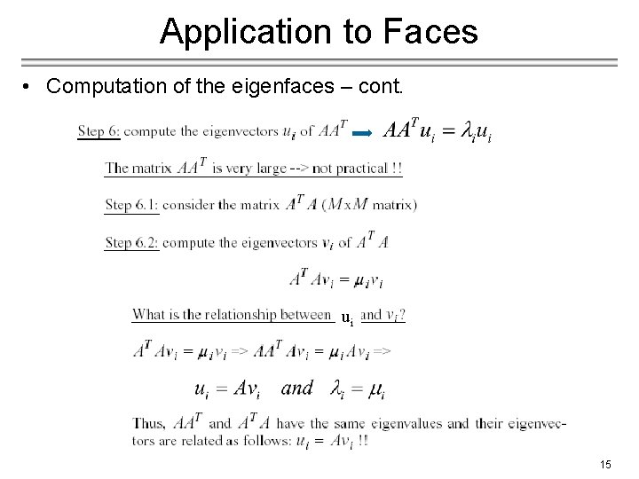
Application to Faces • Computation of the eigenfaces – cont. ui 15

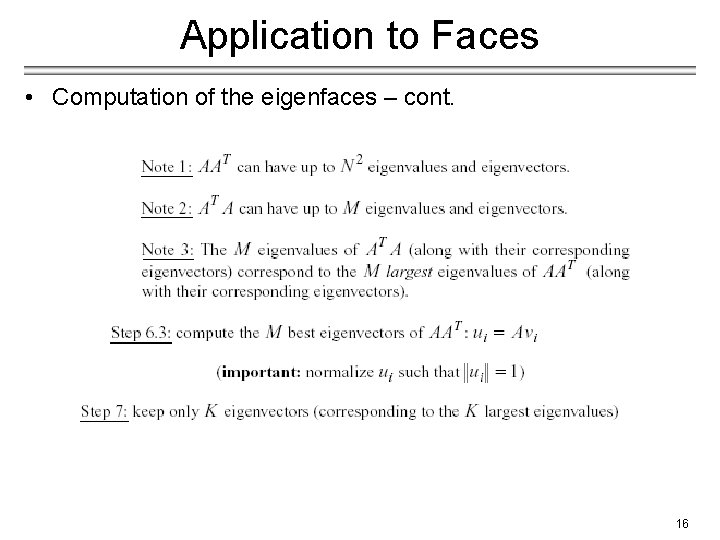
Application to Faces • Computation of the eigenfaces – cont. 16

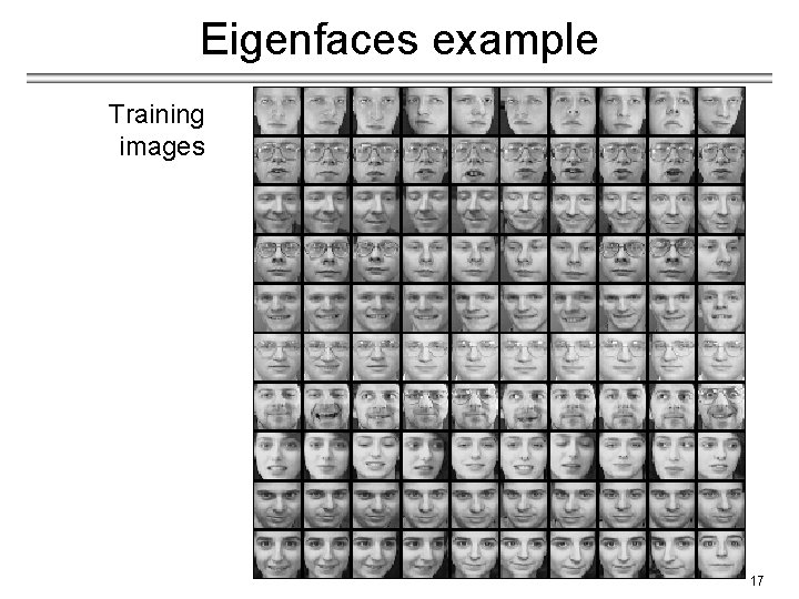
Eigenfaces example Training images 17

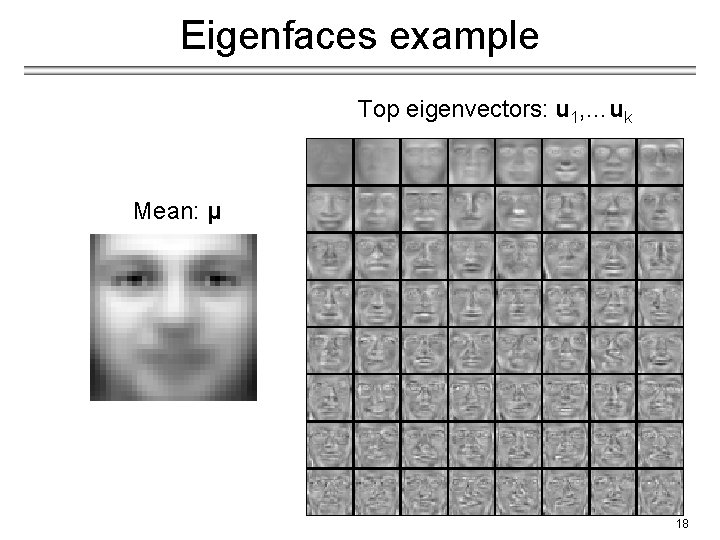
Eigenfaces example Top eigenvectors: u 1, …uk Mean: μ 18

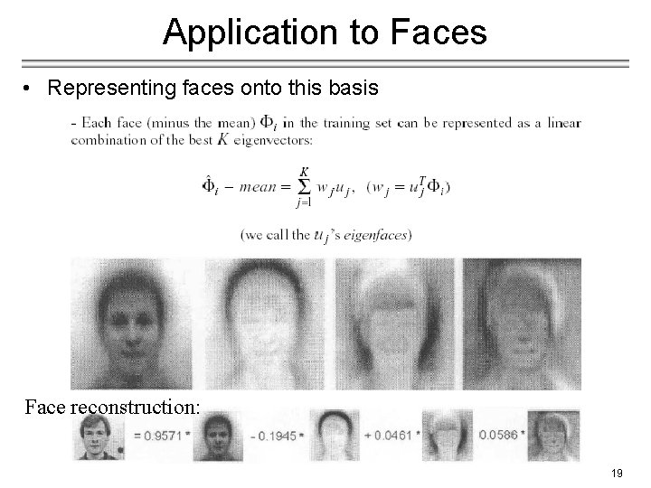
Application to Faces • Representing faces onto this basis Face reconstruction: 19

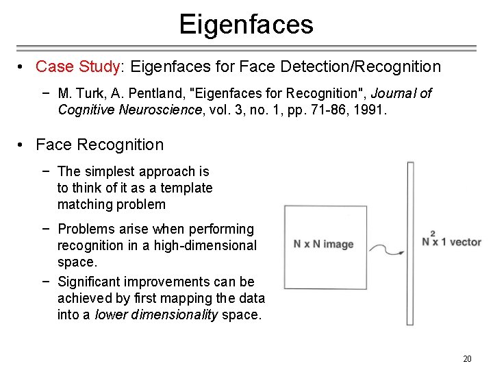
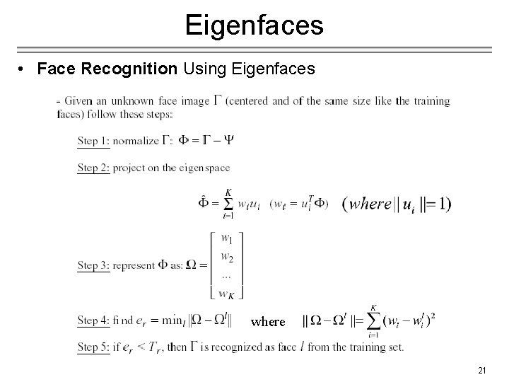
Eigenfaces • Case Study: Eigenfaces for Face Detection/Recognition − M. Turk, A. Pentland, "Eigenfaces for Recognition", Journal of Cognitive Neuroscience, vol. 3, no. 1, pp. 71 -86, 1991. • Face Recognition − The simplest approach is to think of it as a template matching problem − Problems arise when performing recognition in a high-dimensional space. − Significant improvements can be achieved by first mapping the data into a lower dimensionality space. 20

Eigenfaces • Face Recognition Using Eigenfaces where 21

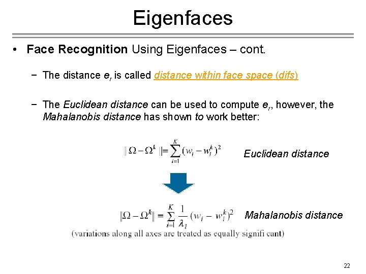
Eigenfaces • Face Recognition Using Eigenfaces – cont. − The distance er is called distance within face space (difs) − The Euclidean distance can be used to compute er, however, the Mahalanobis distance has shown to work better: Euclidean distance Mahalanobis distance 22

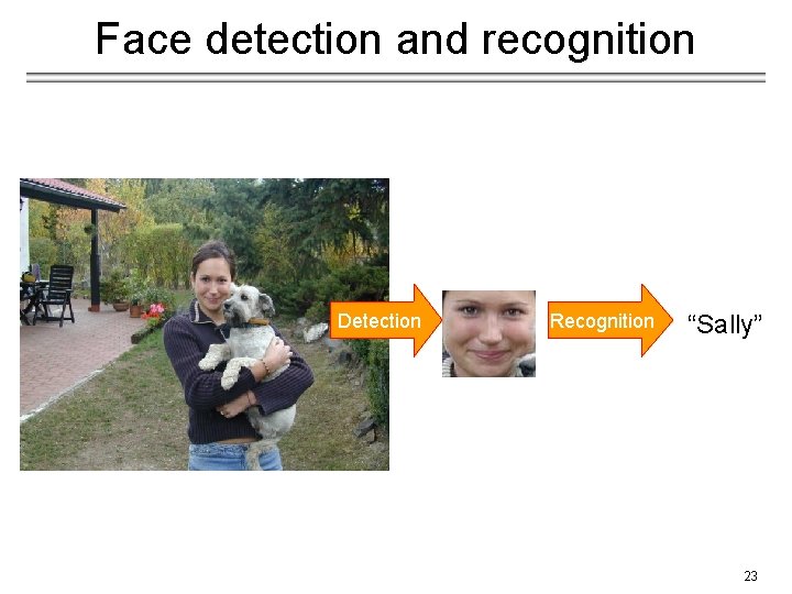
Face detection and recognition Detection Recognition “Sally” 23

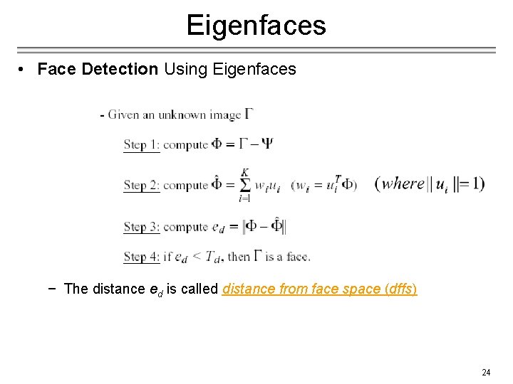
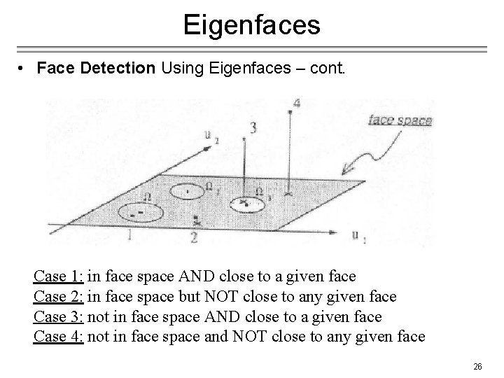
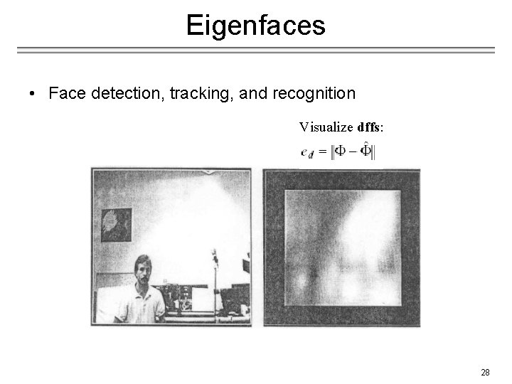
Eigenfaces • Face Detection Using Eigenfaces − The distance ed is called distance from face space (dffs) 24

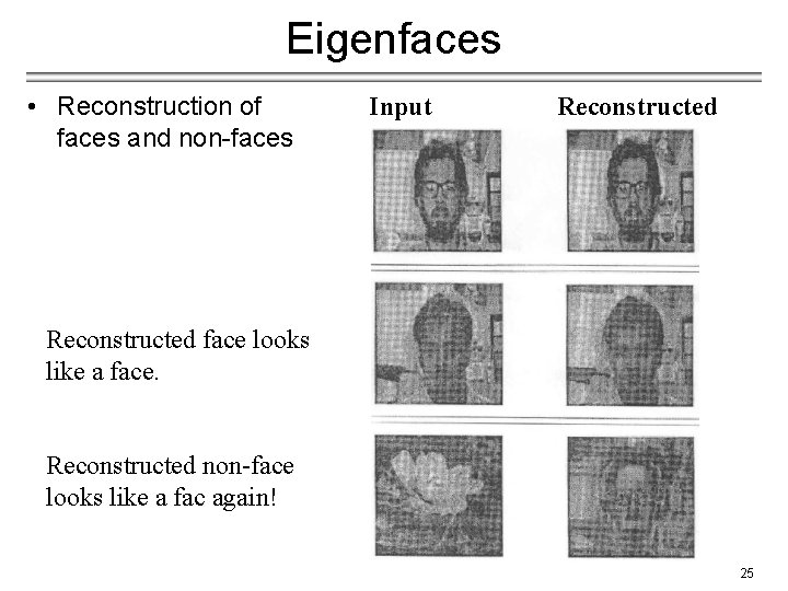
Eigenfaces • Reconstruction of faces and non-faces Input Reconstructed face looks like a face. Reconstructed non-face looks like a fac again! 25

Eigenfaces • Face Detection Using Eigenfaces – cont. Case 1: in face space AND close to a given face Case 2: in face space but NOT close to any given face Case 3: not in face space AND close to a given face Case 4: not in face space and NOT close to any given face 26

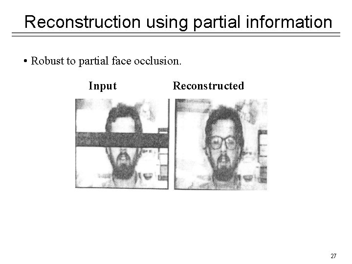
Reconstruction using partial information • Robust to partial face occlusion. Input Reconstructed 27

Eigenfaces • Face detection, tracking, and recognition Visualize dffs: 28

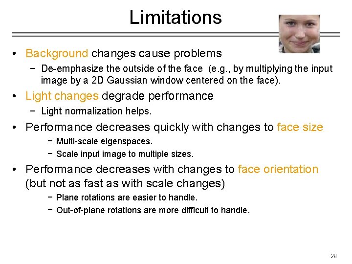
Limitations • Background changes cause problems − De-emphasize the outside of the face (e. g. , by multiplying the input image by a 2 D Gaussian window centered on the face). • Light changes degrade performance − Light normalization helps. • Performance decreases quickly with changes to face size − Multi-scale eigenspaces. − Scale input image to multiple sizes. • Performance decreases with changes to face orientation (but not as fast as with scale changes) − Plane rotations are easier to handle. − Out-of-plane rotations are more difficult to handle. 29

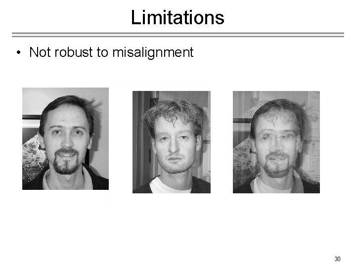
Limitations • Not robust to misalignment 30

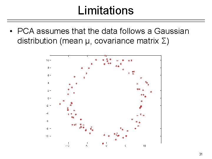
Limitations • PCA assumes that the data follows a Gaussian distribution (mean µ, covariance matrix Σ) The shape of this dataset is not well described by its principal components 31

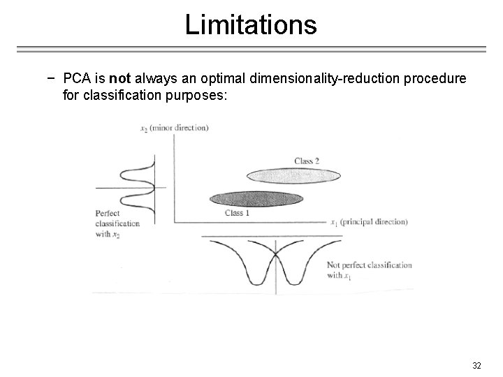
Limitations − PCA is not always an optimal dimensionality-reduction procedure for classification purposes: 32