Image Processing Ch 2 Digital image Fundamentals Prepared

Image Processing Ch 2: Digital image Fundamentals Prepared by: Hanan Hardan

Image sampling and quantization Ch 2: image sampling and quantization p In order to process the image, it must be saved on computer. p The image output of most sensors (eg: Camera) is continuous voltage waveform. p But computer deals with digital images not with continuous images, thus: continuous images should be converted into digital form. continuous image (in real life) digital (computer)

Image sampling and quantization Ch 2: image sampling and quantization

Ch 2: image sampling and quantization Image sampling and quantization continuous image (in real life) digital (computer) To do this we use Two processes: sampling and quantization. Remember that: the image is a function f(x, y), �� x and y are coordinates �� F: intensity value (Amplitude) Sampling: digitizing the coordinate values Quantization: digitizing the amplitude values Thus, when x, y and f are all finite, discrete quantities, we call the image a digital image.

Ch 2: image sampling and quantization How does the computer digitize the continuous image?

Ch 2: image sampling and quantization How does the computer digitize the continuous image? Ex: scan as as ABAB from thethe continuous image, and represent scanaalinesuch from continuous image, and represent the gray intensities.

Ch 2: image sampling and quantization How does the computer digitize the continuous image? Sampling: digitizing coordinates Quantization: digitizing intensities Gray-level scale that divides gray-level into 8 discrete levels Quantization: converting each sample graylevel value into discrete digital quantity. sample is a small white square, located by a vertical tick mark as a point x, y

Ch 2: image sampling and quantization How does the computer digitize the continuous image? Now: the digital scanned line AB representation on computer: The continuous image VS the result of digital image after sampling and quantization

Ch 2: image sampling and quantization Representing digital images Every pixel has a # of bits.

Digital Image Representation Coordinate Conventions p p The result of sampling and quantization is a matrix of real numbers There are two principle ways to represent a digital image: n Assume that an image f(x, y) is sampled so that the resulting image has M rows and N columns. We say that the image is of size M x N. The values of the coordinates (x, y) are discrete quantities. For clarity, we use integer values for these discrete coordinates. In many image processing books, the image origin is defined to be at (x, y) = (0, 0). The next coordinate values along the first row of the image are (x, y) = (0, 1). It is important to keep in mind that the notation (0, 1) is used to signify the second sample along the first row. It does not mean that these are the actual values of physical coordinates. Note that x ranges from 0 to M-1, and y ranges from 0 to N-1. Figure (a)

Digital Image Representation Coordinate Conventions n The coordinate convention used in toolbox to denote arrays is different from the preceding paragraph in two minor ways. Instead of using (x, y) the toolbox uses the notation (r, c) to indicate rows and columns. p The origin of the coordinate system is at (r, c) = (1, 1); thus, r ranges from 1 to M and c from 1 to N, in integer increments. This coordinate convention is shown in Figure (b). p

Digital Image Representation Coordinate Conventions (A) (B)

Digital Image Representation Images as Matrices p The coordination system in figure (A) and the preceding discussion lead to the following representation for a digitized image function:

Digital Image Representation Images as Matrices p p The right side of the equation is a digital image by definition. Each element of this array is called an image element, picture element, pixel or pel. A digital image can be represented naturally as a MATLAB matrix: Where f(1, 1) = f(0, 0). Clearly, the two representations are identical, except for the shift in origin.

Ch 2: image sampling and quantization Pixels! p p Every pixel has # of bits (k) Q: Suppose a pixel has 1 bit, how many gray levels can it represent? Answer: 2 intensity levels only, black and white. Bit (0, 1) 0: black , 1: white p Q: Suppose a pixel has 2 bit, how many gray levels can it represent? Answer: 4 gray intensity levels 2 Bit (00, 01, 10 , 11). Now. . if we want to represent 256 intensities of grayscale, how many bits do we need? Answer: 8 bits which represents: 28=256 so, the gray intensities ( L ) that the pixel can hold, is calculated according to number of pixels it has (k). L= 2 k

Ch 2: image sampling and quantization Number of storage of bits: N * M: the no. of pixels in all the image. K: no. of bits in each pixel L: grayscale levels the pixel can represent L= 2 K all bits in image= N*N*k

Ch 2: image sampling and quantization Number of storage of bits: EX: Here: N=32, K=3, L = 23 =8 # of pixels=N*N = 1024. (because in this example: M=N) # of bits = N*N*K = 1024*3= 3072 N=M in this table, which means no. of horizontal pixels= no. of vertical pixels. And thus: # of pixels in the image= N*N

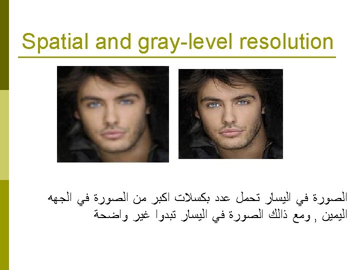
Ch 2: image sampling and quantization Spatial and gray-level resolution Sub sampling Same # of bits in all images (same gray level) different # of pixels sub. Sampling is performed by deleting rows and columns from the original image.

Ch 2: image sampling and quantization Spatial and gray-level resolution Re sampling (pixel replication) A special case of nearest neighbor zooming. Resampling is performed by row and column duplication