Image processing and computer vision Chapter 6 Histogram

Image processing and computer vision Chapter 6: Histogram equalization and color models Histogram, color v. 0. b 1

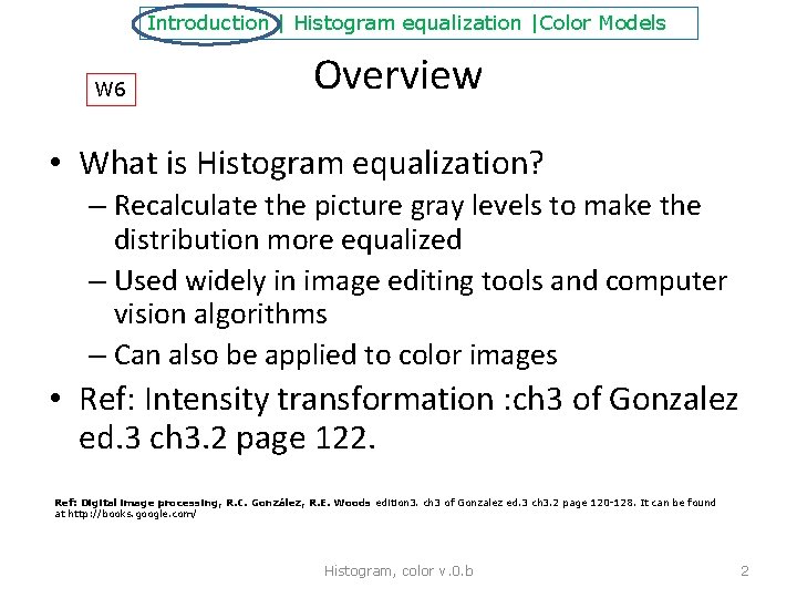
Introduction | Histogram equalization |Color Models W 6 Overview • What is Histogram equalization? – Recalculate the picture gray levels to make the distribution more equalized – Used widely in image editing tools and computer vision algorithms – Can also be applied to color images • Ref: Intensity transformation : ch 3 of Gonzalez ed. 3 ch 3. 2 page 122. Ref: Digital image processing, R. C. González, R. E. Woods edition 3. ch 3 of Gonzalez ed. 3 ch 3. 2 page 120 -128. It can be found at http: //books. google. com/ Histogram, color v. 0. b 2

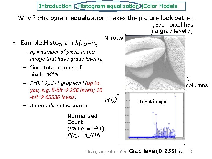
Introduction | Histogram equalization |Color Models Why ? : Histogram equalization makes the picture look better. • Eample: Histogram h(rk)=nk M rows – nk = number of pixels in the image that have grade level rk. – Since total number of pixels=M*N – K=0, 1, 2, . . L-1 gray level (up to you, e. g. 8 -bit 256 levels; 16 -bit 65536 levels) P(rk) – A normalized histogram Each pixel has a gray level rk. N columns Bright image Normalized Count (value =0 1) P(rk)=nk/MN Histogram, color v. 0. b Grad level(0 -255) rk 3

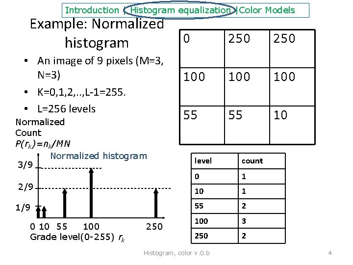
Introduction | Histogram equalization |Color Models Example: Normalized histogram • An image of 9 pixels (M=3, N=3) • K=0, 1, 2, . . , L-1=255. • L=256 levels Normalized Count P(rk)=nk/MN Normalized histogram 3/9 2/9 1/9 0 10 55 100 250 Grade level(0 -255) rk 0 250 100 100 55 55 10 level count 0 1 10 1 55 2 100 3 250 2 Histogram, color v. 0. b 4

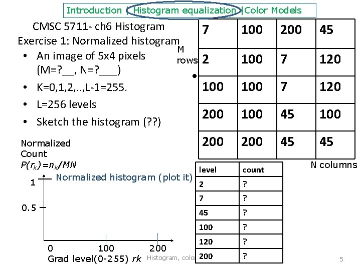
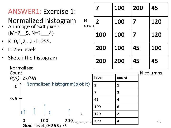
Introduction | Histogram equalization |Color Models CMSC 5711 - ch 6 Histogram Exercise 1: Normalized histogram M • An image of 5 x 4 pixels rows (M=? __, N=? ___) • • K=0, 1, 2, . . , L-1=255. • L=256 levels • Sketch the histogram (? ? ) 7 100 200 45 2 100 7 120 200 100 45 100 200 Normalized Count P(rk)=nk/MN level Normalized histogram (plot it) 1 2 200 45 45 0. 5 count N columns ? 7 ? 45 ? 100 ? 120 0 100 200 Grad level(0 -255) rk Histogram, color v. 0. b ? ? 5

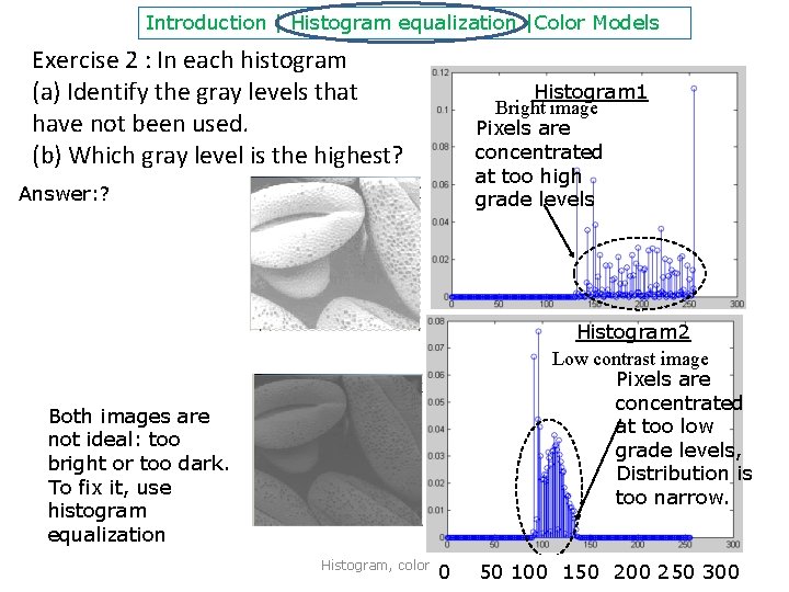
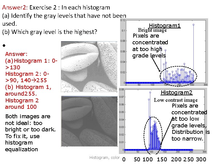
Introduction | Histogram equalization |Color Models Exercise 2 : In each histogram (a) Identify the gray levels that have not been used. (b) Which gray level is the highest? Histogram 1 Bright image Pixels are concentrated at too high grade levels Answer: ? Histogram 2 Low contrast image Pixels are concentrated at too low grade levels, Distribution is too narrow. Both images are not ideal: too bright or too dark. To fix it, use histogram equalization Histogram, color v. 0. b • 0 50 100 150 200 250 3006

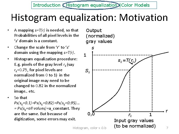
Introduction | Histogram equalization |Color Models Histogram equalization: Motivation • • A mapping s=T(r) is needed, so that Output Probabilities of all pixel levels in the (normalized) ‘s’ domain is a constant. gray values Change the scale from ‘r’ to ‘s’ s domain using the mapping s=T(r). 1 Histogram equalization procedure: sk=T(rk) E. g. pixels of the gray level rk (say rk=0. 75, for pixel levels are Sk normalized from 0 to 1) in the original image may need to be changed to 0. 82 in the normalized image. . etc. So that Ps(sk=0. 1)=Ps(sk=0. 82)=Ps(sk=0. 95). . . = Ps(sk=all values)=a_constant. They are the same. But because of 0, 0 rk 1 digitization, some errors may exit. Input gray values Histogram, color v. 0. b (to be normalized) r 7

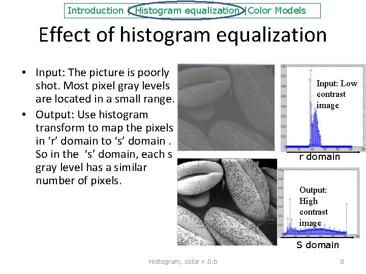
Introduction | Histogram equalization |Color Models Effect of histogram equalization • Input: The picture is poorly shot. Most pixel gray levels are located in a small range. • Output: Use histogram transform to map the pixels in ‘r’ domain to ‘s’ domain. So in the ‘s’ domain, each s gray level has a similar number of pixels. Input: Low contrast image r domain Output: High contrast image S domain Histogram, color v. 0. b 8

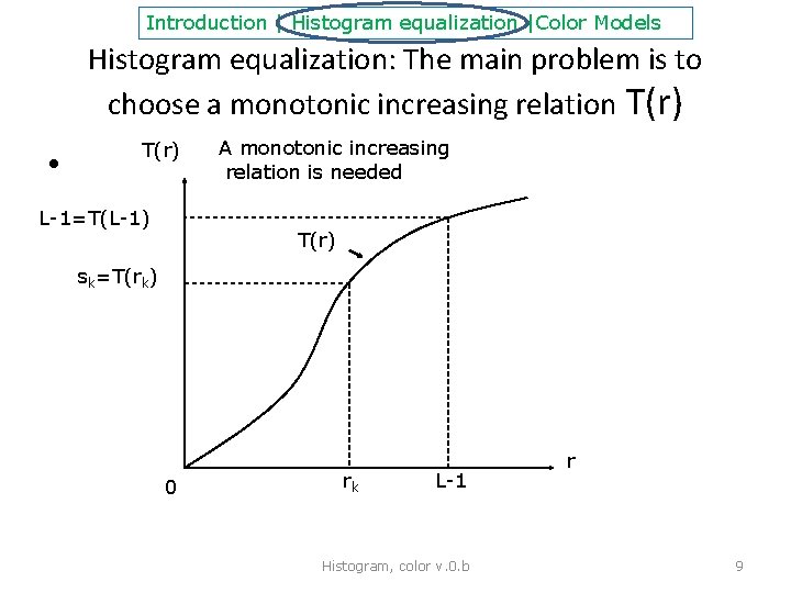
Introduction | Histogram equalization |Color Models Histogram equalization: The main problem is to choose a monotonic increasing relation T(r) • T(r) L-1=T(L-1) A monotonic increasing relation is needed T(r) sk=T(rk) 0 rk L-1 Histogram, color v. 0. b r 9

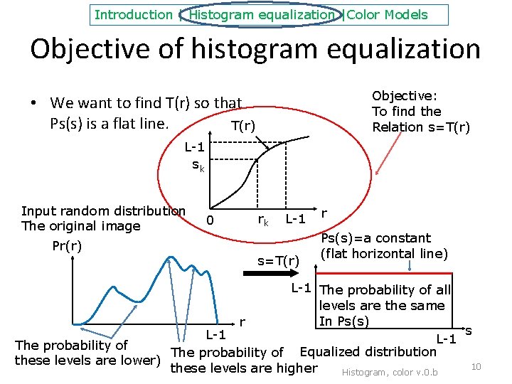
Introduction | Histogram equalization |Color Models Objective of histogram equalization Objective: To find the Relation s=T(r) • We want to find T(r) so that Ps(s) is a flat line. T(r) L-1 sk Input random distribution The original image Pr(r) 0 rk L-1 s=T(r) r Ps(s)=a constant (flat horizontal line) L-1 The probability of all levels are the same In Ps(s) r s L-1 The probability of Equalized distribution these levels are lower) 10 these levels are higher Histogram, color v. 0. b

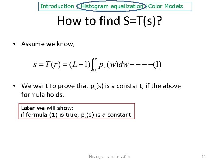
Introduction | Histogram equalization |Color Models How to find S=T(s)? • Assume we know, • We want to prove that ps(s) is a constant, if the above formula holds. Later we will show: if formula (1) is true, ps(s) is a constant Histogram, color v. 0. b 11

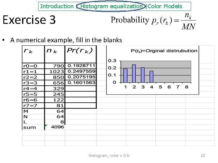
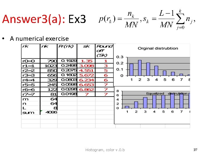
Introduction | Histogram equalization |Color Models Exercise 3 • A numerical example, fill in the blanks Histogram, color v. 0. b 12

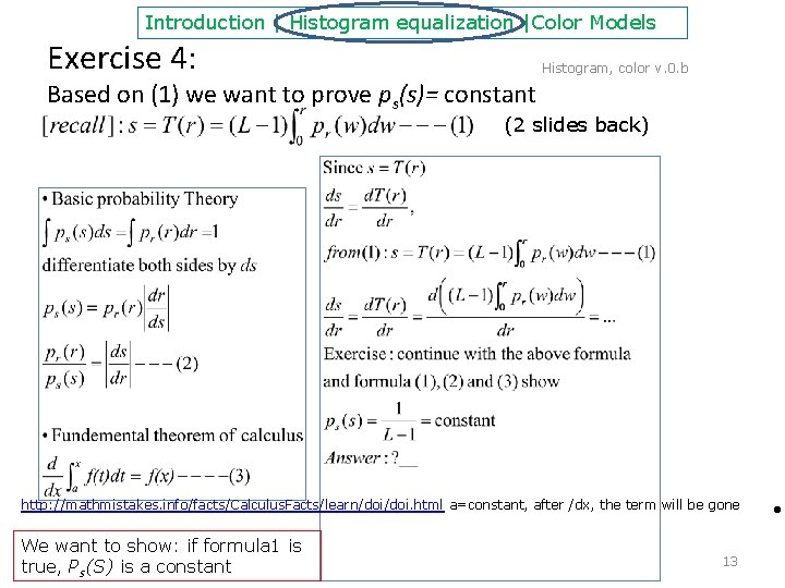
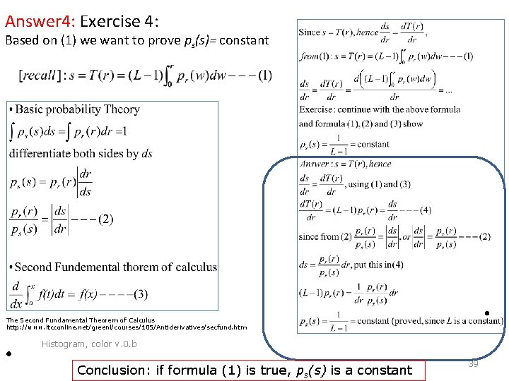
Introduction | Histogram equalization |Color Models Exercise 4: Histogram, color v. 0. b Based on (1) we want to prove ps(s)= constant (2 slides back) http: //mathmistakes. info/facts/Calculus. Facts/learn/doi. html a=constant, after /dx, the term will be gone We want to show: if formula 1 is true, Ps(S) is a constant 13 •

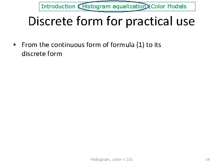
Introduction | Histogram equalization |Color Models Discrete form for practical use • From the continuous form of formula (1) to its discrete form Histogram, color v. 0. b 14

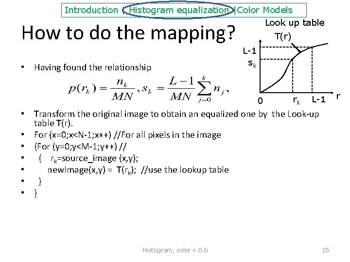
Introduction | Histogram equalization |Color Models Look up table How to do the mapping? • Having found the relationship T(r) L-1 sk 0 rk L-1 • Transform the original image to obtain an equalized one by the Look-up table T(r). • For (x=0; x<N-1; x++) //For all pixels in the image • {For (y=0; y<M-1; y++) // • { rk=source_image (x, y); • new. Image(x, y) = T(rk); //use the lookup table • } • } Histogram, color v. 0. b 15 r

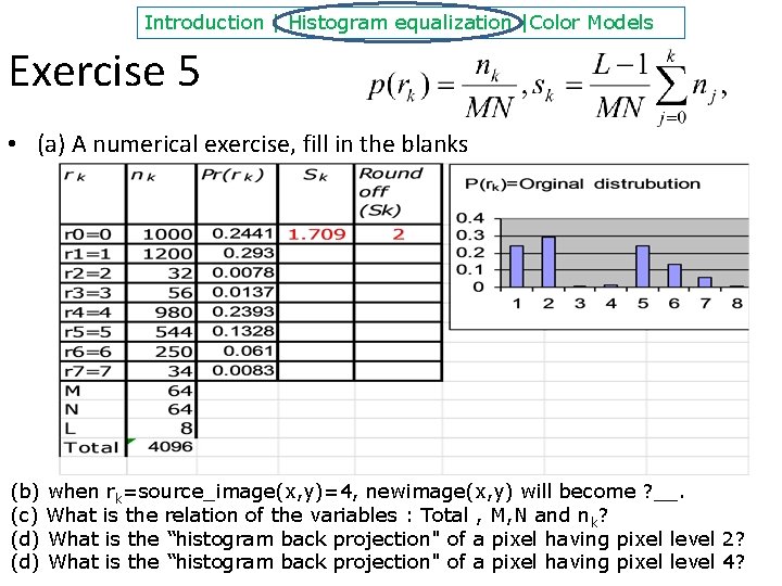
Introduction | Histogram equalization |Color Models Exercise 5 • (a) A numerical exercise, fill in the blanks (b) when rk=source_image(x, y)=4, newimage(x, y) will become ? __. (c) What is the relation of the variables : Total , M, N and n k? (d) What is the “histogram back projection" of a pixel having pixel level 2? Histogram, color v. 0. b 16 (d) What is the “histogram back projection" of a pixel having pixel level 4?

Introduction | Histogram equalization |Color Models Histogram equalization • Most pictures are in color, having multiple color channels. • We need to equalize color pictures • Then, how to represent color images? Histogram, color v. 0. b 17

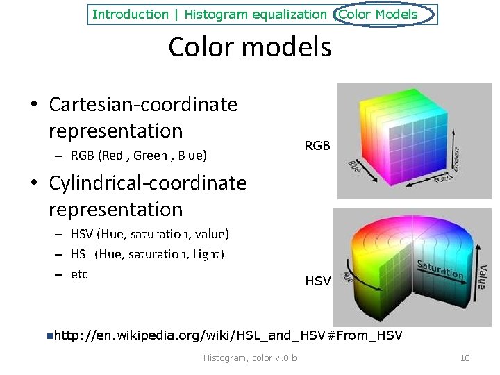
Introduction | Histogram equalization |Color Models Color models • Cartesian-coordinate representation – RGB (Red , Green , Blue) RGB • Cylindrical-coordinate representation – HSV (Hue, saturation, value) – HSL (Hue, saturation, Light) – etc HSV nhttp: //en. wikipedia. org/wiki/HSL_and_HSV#From_HSV Histogram, color v. 0. b 18

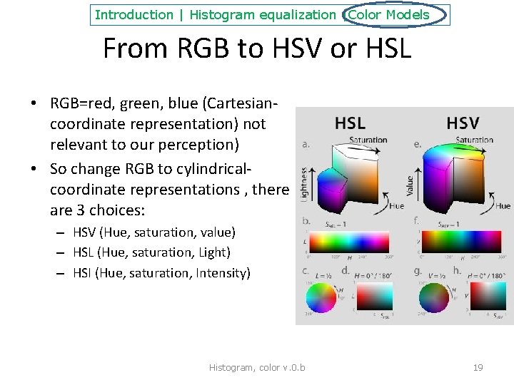
Introduction | Histogram equalization |Color Models From RGB to HSV or HSL • RGB=red, green, blue (Cartesiancoordinate representation) not relevant to our perception) • So change RGB to cylindricalcoordinate representations , there are 3 choices: – HSV (Hue, saturation, value) – HSL (Hue, saturation, Light) – HSI (Hue, saturation, Intensity) Histogram, color v. 0. b 19

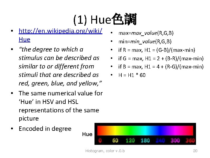
(1) Hue色調 • http: //en. wikipedia. org/wiki/ Hue • “the degree to which a stimulus can be described as similar to or different from stimuli that are described as red, green, blue, and yellow, ” • The same numerical value for ‘Hue’ in HSV and HSL representations of the same picture • Encoded in degree • • • max=max_value(R, G, B) min=min_value(R, G, B) if R = max, H 1 = (G-B)/(max-min) if G = max, H 1 = 2 + (B-R)/(max-min) if B = max, H 1 = 4 + (R-G)/(max-min) H = H 1 * 60 Hue Histogram, color v. 0. b 20

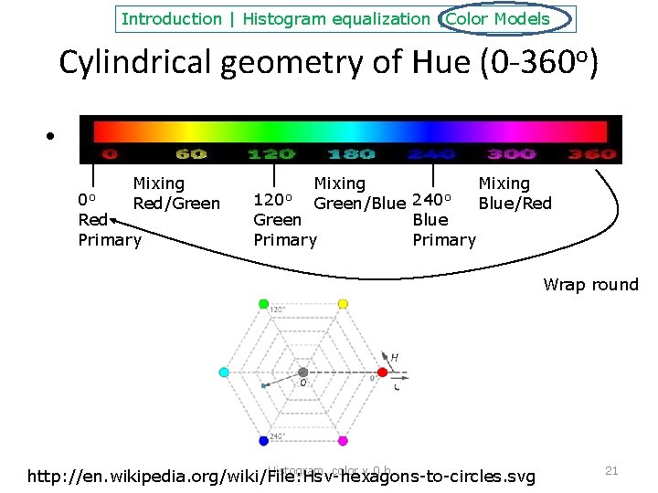
Introduction | Histogram equalization |Color Models Cylindrical geometry of Hue (0 -360 o) • Mixing Red/Green 0 o Red Primary Mixing 120 o Green/Blue 240 o Blue/Red Green Blue Primary Wrap round Histogram, color v. 0. b http: //en. wikipedia. org/wiki/File: Hsv-hexagons-to-circles. svg 21

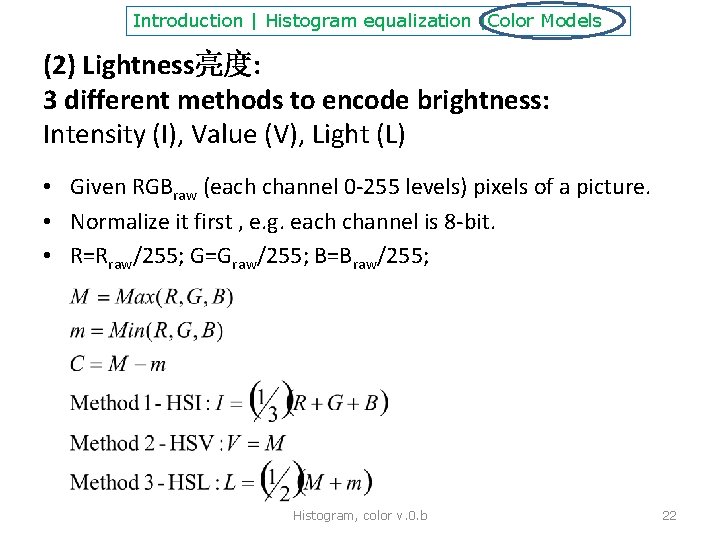
Introduction | Histogram equalization |Color Models (2) Lightness亮度: 3 different methods to encode brightness: Intensity (I), Value (V), Light (L) • Given RGBraw (each channel 0 -255 levels) pixels of a picture. • Normalize it first , e. g. each channel is 8 -bit. • R=Rraw/255; G=Graw/255; B=Braw/255; Histogram, color v. 0. b 22

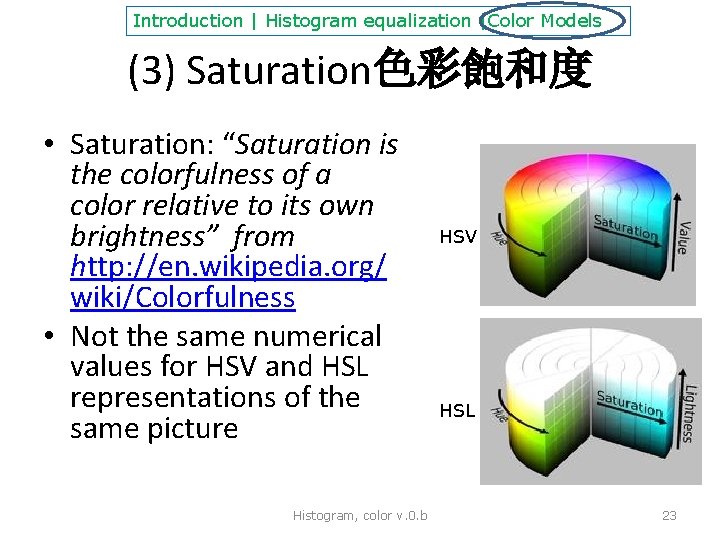
Introduction | Histogram equalization |Color Models (3) Saturation色彩飽和度 • Saturation: “Saturation is the colorfulness of a color relative to its own brightness” from http: //en. wikipedia. org/ wiki/Colorfulness • Not the same numerical values for HSV and HSL representations of the same picture Histogram, color v. 0. b HSV HSL 23

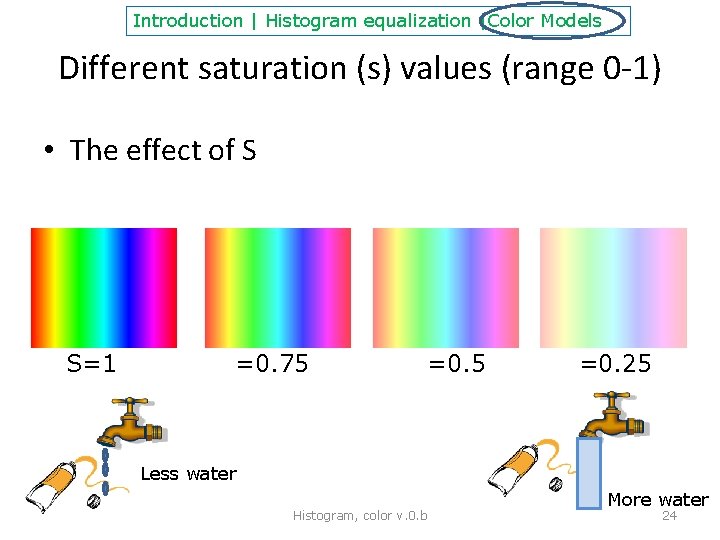
Introduction | Histogram equalization |Color Models Different saturation (s) values (range 0 -1) • The effect of S S=1 =0. 75 =0. 5 =0. 25 Less water Histogram, color v. 0. b More water 24

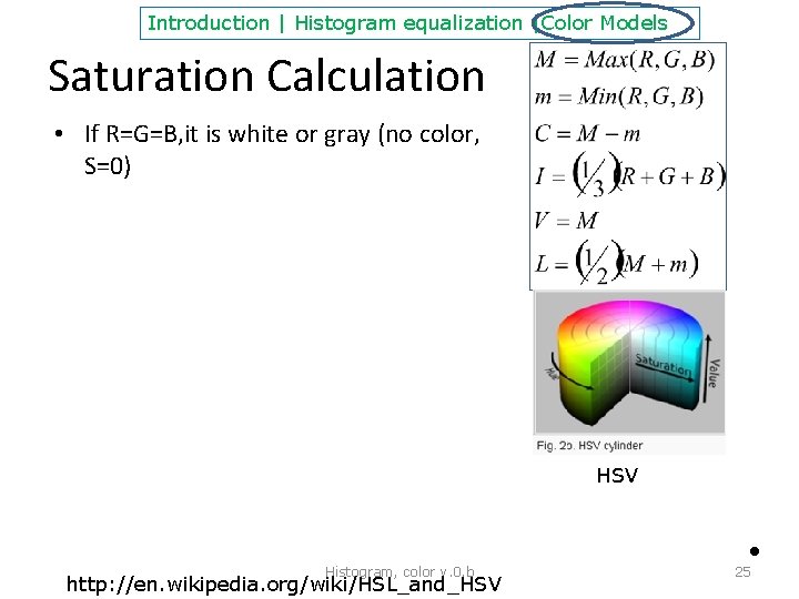
Introduction | Histogram equalization |Color Models Saturation Calculation • If R=G=B, it is white or gray (no color, S=0) HSV Histogram, color v. 0. b http: //en. wikipedia. org/wiki/HSL_and_HSV • 25

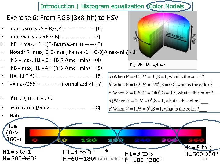
Introduction | Histogram equalization |Color Models Exercise 6: From RGB (3 x 8 -bit) to HSV • • max= max_value(R, G, B) ---------(1) min=min_value(R, G, B) ----------(2) if R = max, H 1 = (G-B)/(max-min) -------(3) Note: if R =max, G, B <max, hence -1< (G-B)/(max-min) <1 if G = max, H 1 = 2 + (B-R)/(max-min)---(4) if B = max, H 1 = 4 + (R-G)/(max-min) ---(5) H = H 1 * 60 ------------------(6) V=max/255 --------(normalized V)--(7) • if H < 0, H = H + 360 • • s=(max-min)/max--------------(8) Note Hue (0 -> 360 o) H 1=5 to 1 H=300 60 o • H 1=1 to 3 H 1=3 to 5 o Histogram, color v. 0. b H=60 180 H=180 300 o H 1=5 to 1 H=300 60 o 26 •

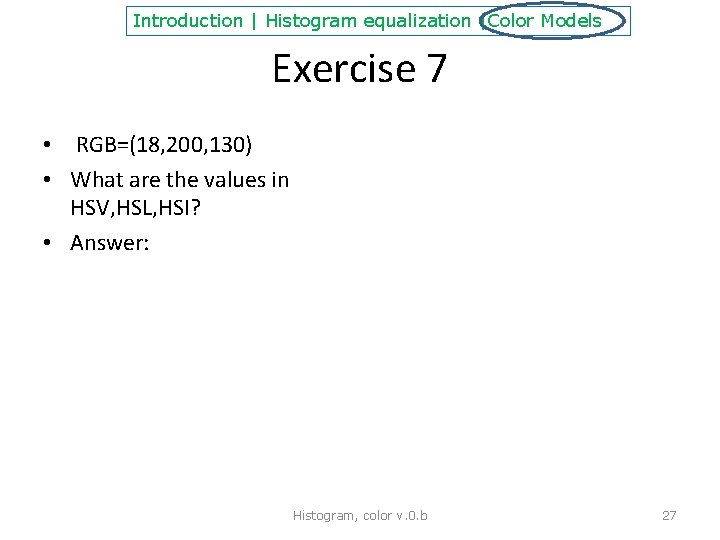
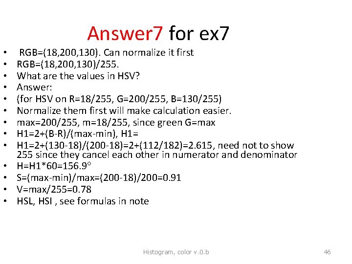
Introduction | Histogram equalization |Color Models Exercise 7 • RGB=(18, 200, 130) • What are the values in HSV, HSL, HSI? • Answer: Histogram, color v. 0. b 27

Introduction | Histogram equalization |Color Models Color histogram equalization • • Change the RGB representation to HSV Do histogram equalization for the V channel. The other two channels (H, S) remain unchanged. Put back the equalized HSV image back to RGB Histogram, color v. 0. b 28

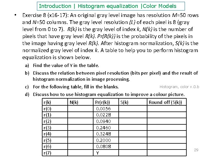
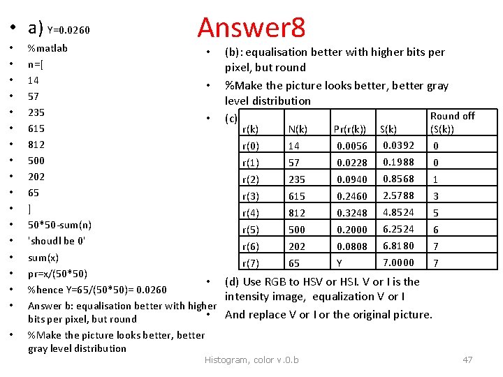
Introduction | Histogram equalization |Color Models • Exercise 8 (x 16 -17): An original gray level image has resolution M=50 rows and N=50 columns. The gray level resolution (L) of each pixel is 8 (gray level from 0 to 7). R(k) is the gray level of index k, N(k) is the number of pixels that have gray level R(k). Pr(R(k)) is the probability of the pixels in the image having gray level R(k). After histogram normalization, S(k) is the normalized gray level of index k. A table to help you to perform histogram equalization is shown below. a) Find the value of Y in the table. b) Discuss the relation between pixel resolution (bits per pixel) and the result of histogram normalization in image processing. Histogram, color v. 0. b c) For the following table, fill in the blanks. d) Discuss how to use histogram equalization to improve a colour picture. r(k) N(k) Pr(r(k)) S(k) Round off (S(k)) r(0) 0. 0056 r(1) 0. 0228 r(2) 0. 0940 r(3) 0. 2460 r(4) 0. 3248 r(5) 0. 2000 r(6) 0. 0808 29 r(7) Y

Introduction | Histogram equalization |Color Models Programs and demos • Histogram in Open. CV: Calculate Histogram: http: //opencv. willowgarage. com/documentation/cpp/histograms. html? h ighlight=calchist#calc. Hist –Convert color space: http: //opencv. willowgarage. com/documentation/cpp/miscellaneous_im age_transformations. html? highlight=cvtcolor#cvt. Color –Histogram equalization http: //opencv. willowgarage. com/documentation/cpp/histograms. html? h ighlight=equalizehist#equalize. Histogram, color v. 0. b 30

Introduction | Histogram equalization |Color Models Programming Exercise • A programming exercise with Open. CV to histogram equalize a color image – Given an RGB color image, convert it to HSV color space, compute its histogram on the V channel – Do histogram equalization for the V channel and generate the equalized RGB image. Histogram, color v. 0. b 31

Summary • Studied gray level histograms • Learned histogram equalization • Learned color models and equalization of color images Histogram, color v. 0. b 32

Reference • Digital image processing, R. C. González, R. E. Woods edition 3. ch 3 of Gonzalez ed. 3 ch 3. 2 page 120 -128. It can be found at http: //books. google. com/ • http: //en. wikipedia. org/wiki/Histogram_equal ization Histogram, color v. 0. b 33

Appendix • Histogram, color v. 0. b 34

ANSWER 1: Exercise 1: Normalized histogram • An image of 5 x 4 pixels (M=? __5, N=? ___4) • K=0, 1, 2, . . , L-1=255. • L=256 levels • Sketch the histogram M rows Normalized Count P(rk)=nk/MN Normalized histogram(plot it) 1 0. 5 7 100 200 45 2 100 7 120 100 • 100 7 120 200 100 45 100 200 45 45 level count 2 1 7 3 45 4 100 6 120 2 0 100 200 Histogram, color v. 0. b Grad level(0 -255) rk 4 N columns 35

Answer 2: Exercise 2 : In each histogram (a) Identify the gray levels that have not been used. (b) Which gray level is the highest? • Answer: (a)Histogram 1: 0>130 Histogram 2: 0>90, 140 255 (b) Histogram 1, around 255. Histogram 2 around 100 Histogram 1 Bright image Pixels are concentrated at too high grade levels Histogram 2 Low contrast image Pixels are concentrated at too low grade levels, Distribution is too narrow. Both images are not ideal: too bright or too dark. To fix it, use histogram equalization Histogram, color v. 0. b 36 0 50 100 150 200 250 300

Answer 3(a): Ex 3 • A numerical exercise Histogram, color v. 0. b 37 37

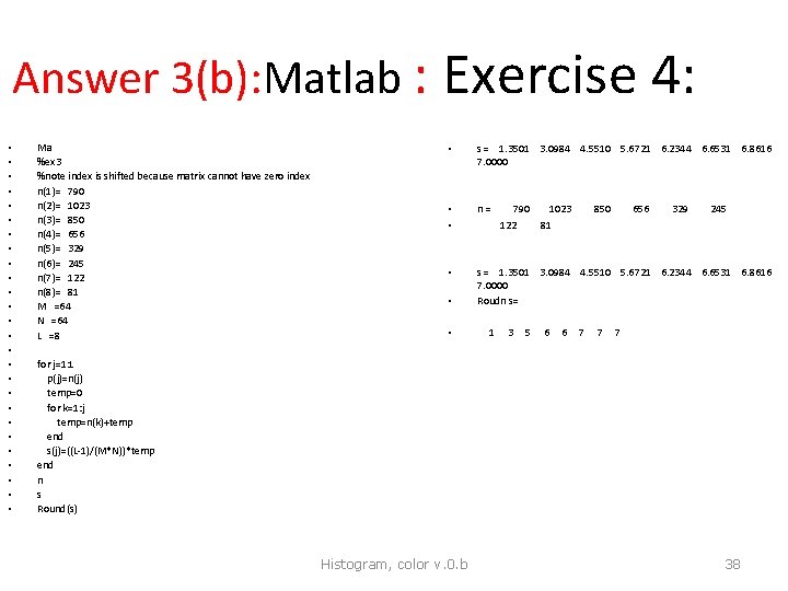
Answer 3(b): Matlab : Exercise 4: • • • • • • • Ma %ex 3 %note index is shifted because matrix cannot have zero index n(1)= 790 n(2)= 1023 n(3)= 850 n(4)= 656 n(5)= 329 n(6)= 245 n(7)= 122 n(8)= 81 M =64 N =64 L =8 for j=1: L p(j)=n(j) temp=0 for k=1: j temp=n(k)+temp end s(j)=((L-1)/(M*N))*temp end n s Round(s) • s = 1. 3501 3. 0984 4. 5510 5. 6721 6. 2344 6. 6531 6. 8616 7. 0000 • • n = 790 1023 850 656 329 245 122 81 • • s = 1. 3501 3. 0984 4. 5510 5. 6721 6. 2344 6. 6531 6. 8616 7. 0000 Roudn s= • 1 3 5 6 6 7 7 7 Histogram, color v. 0. b 38

Answer 4: Exercise 4: Based on (1) we want to prove ps(s)= constant • The Second Fundamental Theorem of Calculus http: //www. ltcconline. net/greenl/courses/105/Antiderivatives/secfund. htm • Histogram, color v. 0. b Conclusion: if formula (1) is true, ps(s) is a constant 39

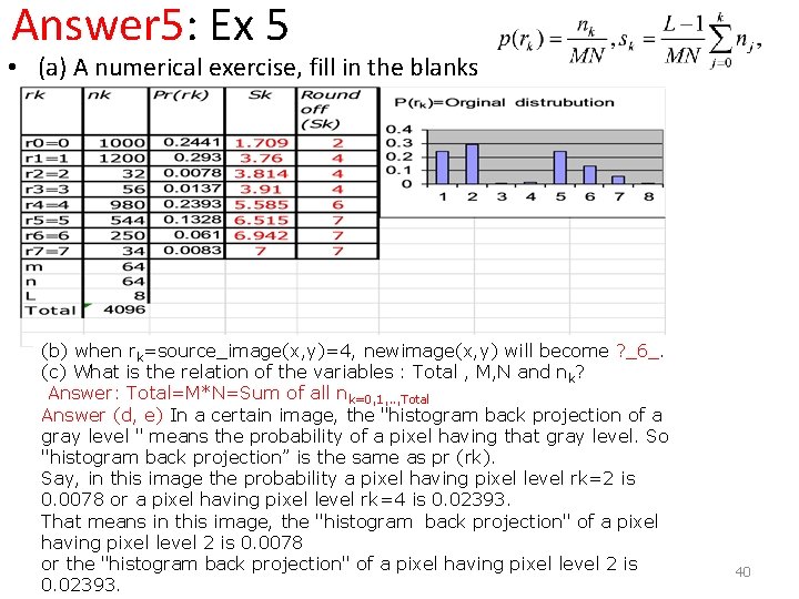
Answer 5: Ex 5 • (a) A numerical exercise, fill in the blanks (b) when rk=source_image(x, y)=4, newimage(x, y) will become ? _6_. (c) What is the relation of the variables : Total , M, N and n k? Answer: Total=M*N=Sum of all nk=0, 1, . . , Total Answer (d, e) In a certain image, the "histogram back projection of a gray level " means the probability of a pixel having that gray level. So "histogram back projection” is the same as pr (rk). Say, in this image the probability a pixel having pixel level rk=2 is 0. 0078 or a pixel having pixel level rk=4 is 0. 02393. That means in this image, the "histogram back projection" of a pixel having pixel level 2 is 0. 0078 or the "histogram back projection" of a pixel having pixel level 2 is Histogram, color v. 0. b 0. 02393. 40

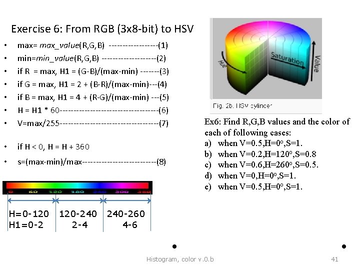
Exercise 6: From RGB (3 x 8 -bit) to HSV • • max= max_value(R, G, B) ---------(1) min=min_value(R, G, B) ----------(2) if R = max, H 1 = (G-B)/(max-min) -------(3) if G = max, H 1 = 2 + (B-R)/(max-min)---(4) if B = max, H 1 = 4 + (R-G)/(max-min) ---(5) H = H 1 * 60 ------------------(6) V=max/255 ------------------(7) • if H < 0, H = H + 360 • s=(max-min)/max--------------(8) Ex 6: Find R, G, B values and the color of each of following cases: a) when V=0. 5, H=0 o, S=1. b) when V=0. 2, H=120 o, S=0. 8 c) when V=0. 6, H=260 o, S=0. 5. d) when V=0, H=0 o, S=1. e) when V=0. 5, H=0 o, S=1. H=0 -120 120 -240 240 -260 H 1=0 -2 2 -4 4 -6 • Histogram, color v. 0. b 41 •

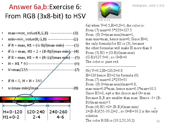
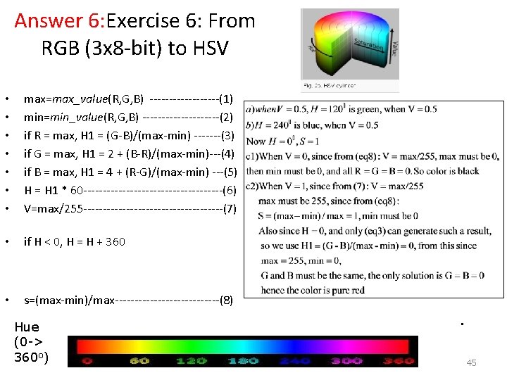
Answer 6 a, b: Exercise 6: From RGB (3 x 8 -bit) to HSV • • max=max_value(R, G, B) ---------(1) min=min_value(R, G, B) ----------(2) if R = max, H 1 = (G-B)/(max-min) -------(3) if G = max, H 1 = 2 + (B-R)/(max-min)---(4) if B = max, H 1 = 4 + (R-G)/(max-min) ---(5) H = H 1 * 60 ------------------(6) V=max/255 ------------------(7) • if H < 0, H = H + 360 • s=(max-min)/max--------------(8) H=0 -120 120 -240 240 -260 H 1=0 -2 2 -4 4 -6 Histogram, color v. 0. b 6 a) when V=0. 5, H=0, S=1, the color is : From (7) max=0. 5*255=127. 5 From (8) S=(max-min)/max=1, max-min=max, hence min=0, Since H=0, the only formula for H 1 is (3), because the other formulas will make H more than 0 From (3) H 1 = (G-B)/(max-min) (G-B)/127. 5=0 , so G=B=0 The color is pure red. --------------------6 b) V=0. 2, H=120, S=0. 8 H=120 hence H 1=2 by formula (6) From (7) max=0. 2*255=51 From (8) S=(max-min)/max=0. 8, max-min=0. 8*max, hence min=0. 2*max=10. 2 Since H 1=2, eq 4 is the choice and G= max. Because B, R are smaller than max. Hence -1< (BR)/(max-min)<1 From (4) H 1 =2+ (B-R)/(max-min) • 2+(B-R)/(51 -10. 2)=2 , so G=B=10. 2 is the only solution The color RGB is (10. 2, 51, 10. 2) 42

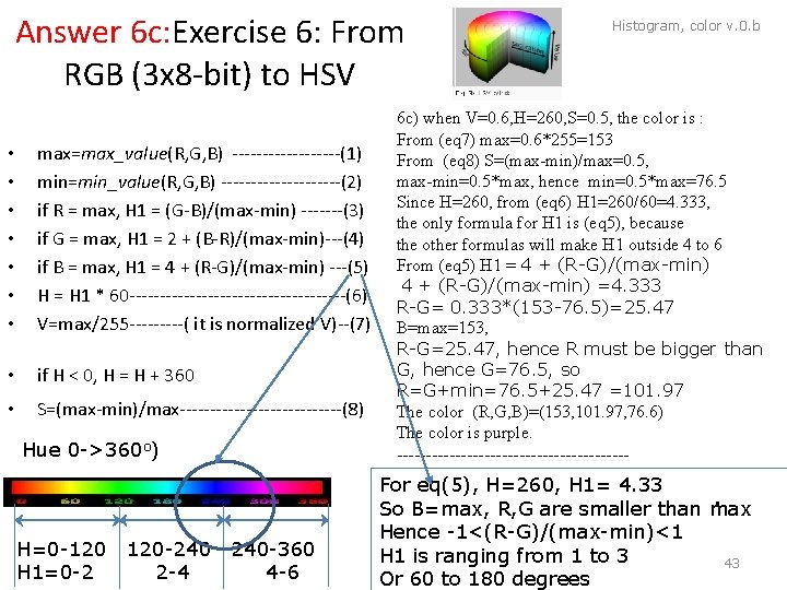
Answer 6 c: Exercise 6: From RGB (3 x 8 -bit) to HSV • • max=max_value(R, G, B) ---------(1) min=min_value(R, G, B) ----------(2) if R = max, H 1 = (G-B)/(max-min) -------(3) if G = max, H 1 = 2 + (B-R)/(max-min)---(4) if B = max, H 1 = 4 + (R-G)/(max-min) ---(5) H = H 1 * 60 ------------------(6) V=max/255 -----( it is normalized V)--(7) • if H < 0, H = H + 360 • S=(max-min)/max--------------(8) Hue 0 ->360 o) H=0 -120 120 -240 240 -360 H 1=0 -2 2 -4 4 -6 Histogram, color v. 0. b 6 c) when V=0. 6, H=260, S=0. 5, the color is : From (eq 7) max=0. 6*255=153 From (eq 8) S=(max-min)/max=0. 5, max-min=0. 5*max, hence min=0. 5*max=76. 5 Since H=260, from (eq 6) H 1=260/60=4. 333, the only formula for H 1 is (eq 5), because the other formulas will make H 1 outside 4 to 6 From (eq 5) H 1 = 4 + (R-G)/(max-min) =4. 333 R-G= 0. 333*(153 -76. 5)=25. 47 B=max=153, R-G=25. 47, hence R must be bigger than G, hence G=76. 5, so R=G+min=76. 5+25. 47 =101. 97 The color (R, G, B)=(153, 101. 97, 76. 6) The color is purple. -------------------- For eq(5), H=260, H 1= 4. 33 • So B=max, R, G are smaller than max Hence -1<(R-G)/(max-min)<1 H 1 is ranging from 1 to 3 43 Or 60 to 180 degrees

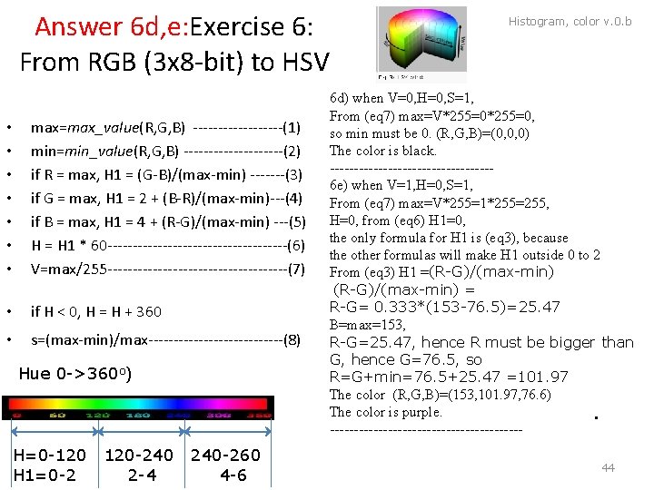
Answer 6 d, e: Exercise 6: From RGB (3 x 8 -bit) to HSV • • max=max_value(R, G, B) ---------(1) min=min_value(R, G, B) ----------(2) if R = max, H 1 = (G-B)/(max-min) -------(3) if G = max, H 1 = 2 + (B-R)/(max-min)---(4) if B = max, H 1 = 4 + (R-G)/(max-min) ---(5) H = H 1 * 60 ------------------(6) V=max/255 ------------------(7) • if H < 0, H = H + 360 • s=(max-min)/max--------------(8) Hue 0 ->360 o) H=0 -120 120 -240 240 -260 H 1=0 -2 2 -4 4 -6 Histogram, color v. 0. b 6 d) when V=0, H=0, S=1, From (eq 7) max=V*255=0, so min must be 0. (R, G, B)=(0, 0, 0) The color is black. -----------------6 e) when V=1, H=0, S=1, From (eq 7) max=V*255=1*255=255, H=0, from (eq 6) H 1=0, the only formula for H 1 is (eq 3), because the other formulas will make H 1 outside 0 to 2 From (eq 3) H 1 =(R-G)/(max-min) = R-G= 0. 333*(153 -76. 5)=25. 47 B=max=153, R-G=25. 47, hence R must be bigger than G, hence G=76. 5, so R=G+min=76. 5+25. 47 =101. 97 The color (R, G, B)=(153, 101. 97, 76. 6) The color is purple. • --------------------44

Answer 6: Exercise 6: From RGB (3 x 8 -bit) to HSV • • max=max_value(R, G, B) ---------(1) min=min_value(R, G, B) ----------(2) if R = max, H 1 = (G-B)/(max-min) -------(3) if G = max, H 1 = 2 + (B-R)/(max-min)---(4) if B = max, H 1 = 4 + (R-G)/(max-min) ---(5) H = H 1 * 60 ------------------(6) V=max/255 ------------------(7) • if H < 0, H = H + 360 • s=(max-min)/max--------------(8) Hue (0 -> 360 o) • Histogram, color v. 0. b 45

Answer 7 for ex 7 • • • • RGB=(18, 200, 130). Can normalize it first RGB=(18, 200, 130)/255. What are the values in HSV? Answer: (for HSV on R=18/255, G=200/255, B=130/255) Normalize them first will make calculation easier. max=200/255, m=18/255, since green G=max H 1=2+(B-R)/(max-min), H 1=2+(130 -18)/(200 -18)=2+(112/182)=2. 615, need not to show 255 since they cancel each other in numerator and denominator H=H 1*60=156. 9 S=(max-min)/max=(200 -18)/200=0. 91 V=max/255=0. 78 HSL, HSI , see formulas in note Histogram, color v. 0. b 46

• a) Y=0. 0260 • • • • • Answer 8 %matlab • n=[ 14 • 57 235 • 615 812 500 202 65 ] 50*50 -sum(n) 'shoudl be 0' sum(x) pr=x/(50*50) • %hence Y=65/(50*50)= 0. 0260 Answer b: equalisation better with higher • bits per pixel, but round %Make the picture looks better, better gray level distribution (b): equalisation better with higher bits per pixel, but round %Make the picture looks better, better gray level distribution Round off (c) r(k) r(0) r(1) r(2) r(3) r(4) r(5) r(6) r(7) N(k) 14 57 235 615 812 500 202 65 Pr(r(k)) 0. 0056 0. 0228 0. 0940 0. 2460 0. 3248 0. 2000 0. 0808 Y S(k) 0. 0392 0. 1988 0. 8568 2. 5788 4. 8524 6. 2524 6. 8180 7. 0000 (S(k)) 0 0 1 3 5 6 7 7 (d) Use RGB to HSV or HSI. V or I is the intensity image, equalization V or I And replace V or I or the original picture. Histogram, color v. 0. b 47