Image Enhancement and Filtering Techniques EE 4 H

Image Enhancement and Filtering Techniques EE 4 H, M. Sc 0407191 Computer Vision Dr. Mike Spann m. spann@bham. ac. uk http: //www. eee. bham. ac. uk/spannm

Introduction Images may suffer from the following degradations: Poor contrast due to poor illumination or finite sensitivity of the imaging device Electronic sensor noise or atmospheric disturbances leading to broad band noise Aliasing effects due to inadequate sampling Finite aperture effects or motion leading to spatial

Introduction We will consider simple algorithms for image enhancement based on lookup tables Contrast enhancement We will also consider simple linear filtering algorithms Noise removal

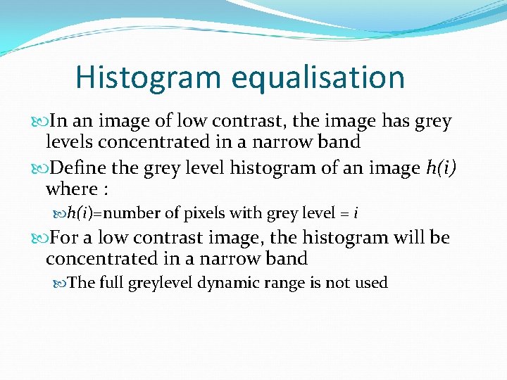
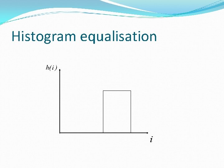
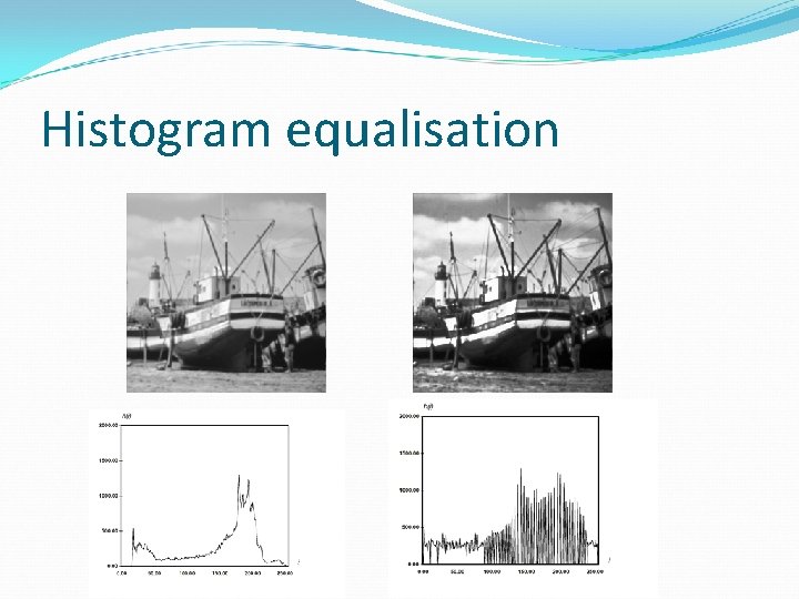
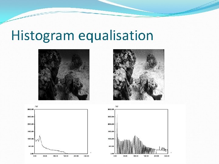
Histogram equalisation In an image of low contrast, the image has grey levels concentrated in a narrow band Define the grey level histogram of an image h(i) where : h(i)=number of pixels with grey level = i For a low contrast image, the histogram will be concentrated in a narrow band The full greylevel dynamic range is not used

Histogram equalisation

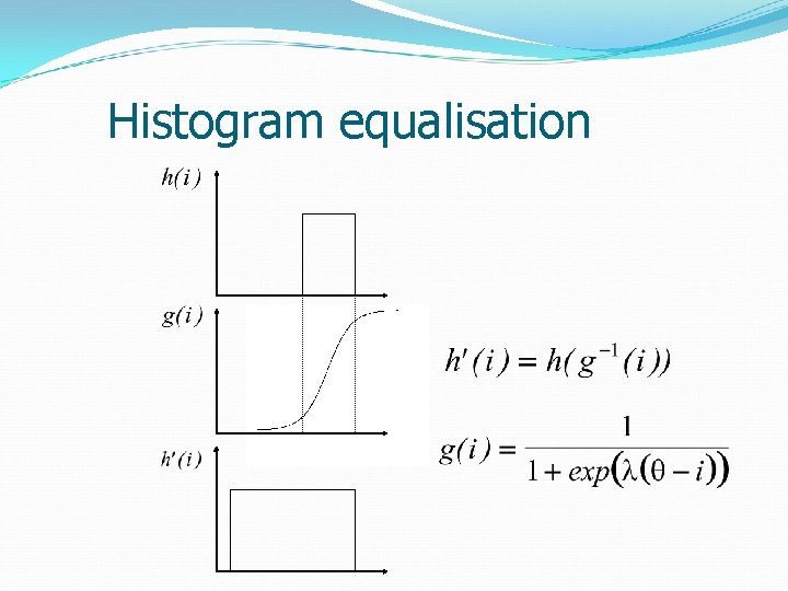
Histogram equalisation Can use a sigmoid lookup to map input to output grey levels A sigmoid function g(i) controls the mapping from input to output pixel Can easily be implemented in hardware for maximum efficiency

Histogram equalisation

Histogram equalisation θ controls the position of maximum slope λ controls the slope Problem - we need to determine the optimum sigmoid parameters and for each image A better method would be to determine the best mapping function from the image data

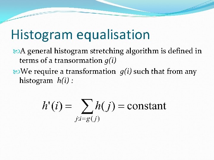
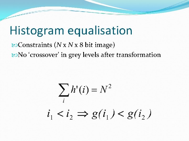
Histogram equalisation A general histogram stretching algorithm is defined in terms of a transormation g(i) We require a transformation g(i) such that from any histogram h(i) :

Histogram equalisation Constraints (N x 8 bit image) No ‘crossover’ in grey levels after transformation

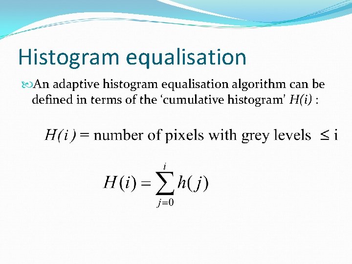
Histogram equalisation An adaptive histogram equalisation algorithm can be defined in terms of the ‘cumulative histogram’ H(i) :

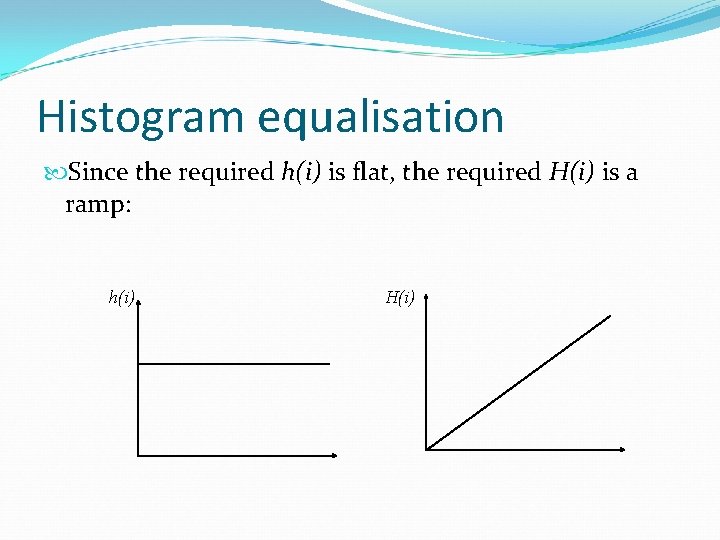
Histogram equalisation Since the required h(i) is flat, the required H(i) is a ramp: h(i) H(i)

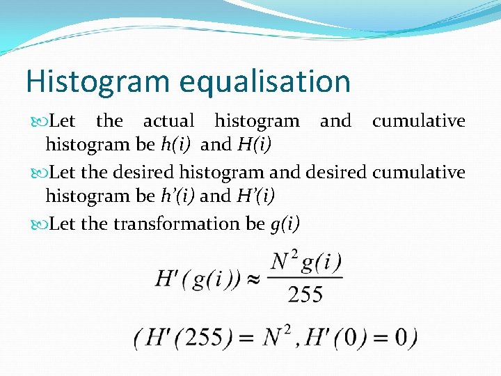
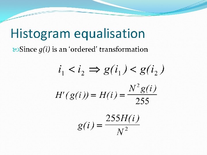
Histogram equalisation Let the actual histogram and cumulative histogram be h(i) and H(i) Let the desired histogram and desired cumulative histogram be h’(i) and H’(i) Let the transformation be g(i)

Histogram equalisation Since g(i) is an ‘ordered’ transformation

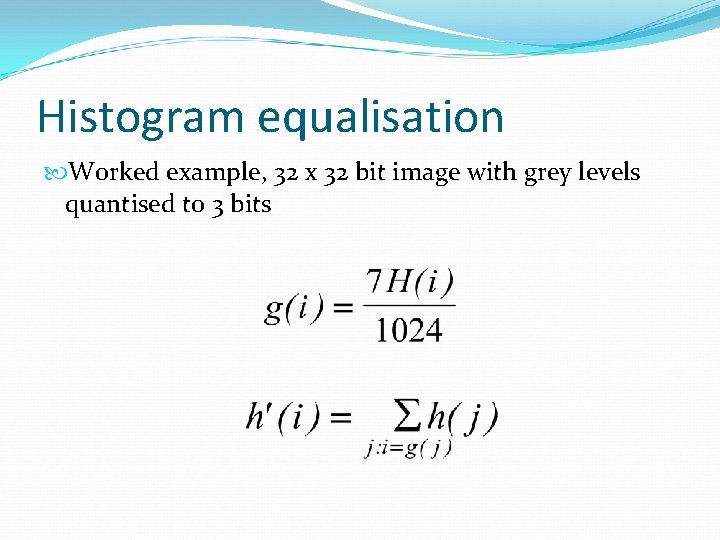
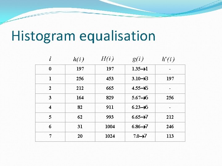
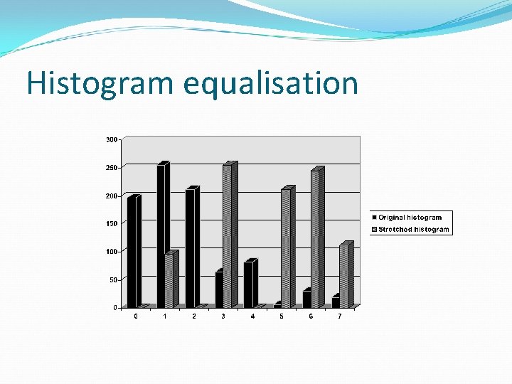
Histogram equalisation Worked example, 32 x 32 bit image with grey levels quantised to 3 bits

Histogram equalisation 0 197 1. 35 1 - 1 256 453 3. 10 3 197 2 212 665 4. 55 5 - 3 164 829 5. 67 6 256 4 82 911 6. 23 6 - 5 62 993 6. 65 7 212 6 31 1004 6. 86 7 246 7 20 1024 7. 0 7 113

Histogram equalisation

Histogram equalisation

Histogram equalisation

Histogram equalisation Image. J demonstration http: //rsb. info. nih. gov/ij/signed-applet

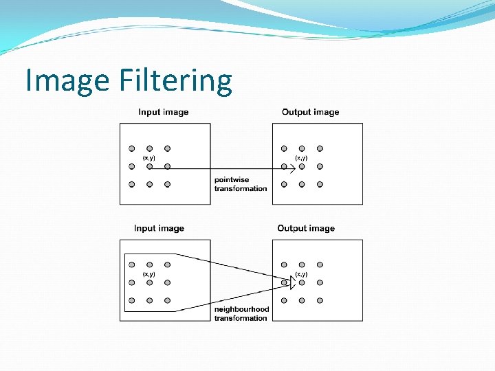
Image Filtering Simple image operators can be classified as 'pointwise' or 'neighbourhood' (filtering) operators Histogram equalisation is a pointwise operation More general filtering operations use neighbourhoods of pixels

Image Filtering

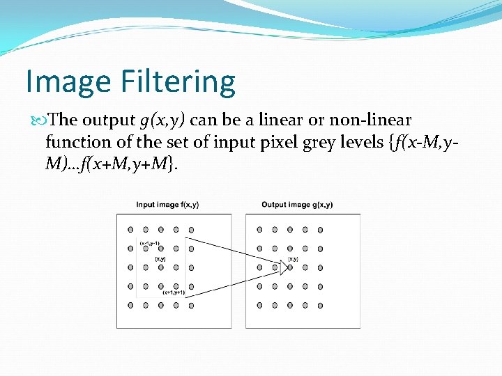
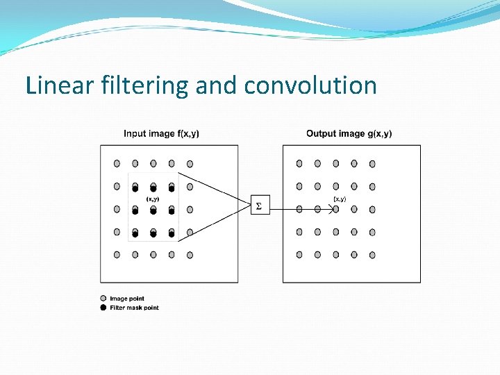
Image Filtering The output g(x, y) can be a linear or non-linear function of the set of input pixel grey levels {f(x-M, y. M)…f(x+M, y+M}.

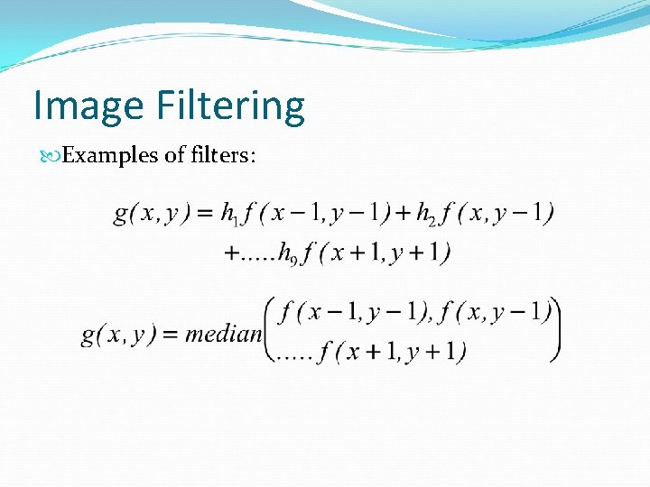
Image Filtering Examples of filters:

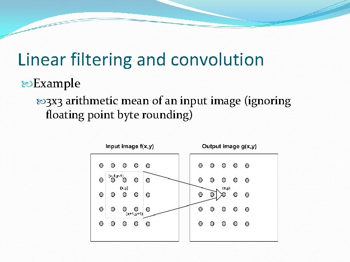
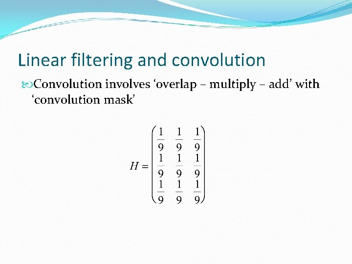
Linear filtering and convolution Example 3 x 3 arithmetic mean of an input image (ignoring floating point byte rounding)

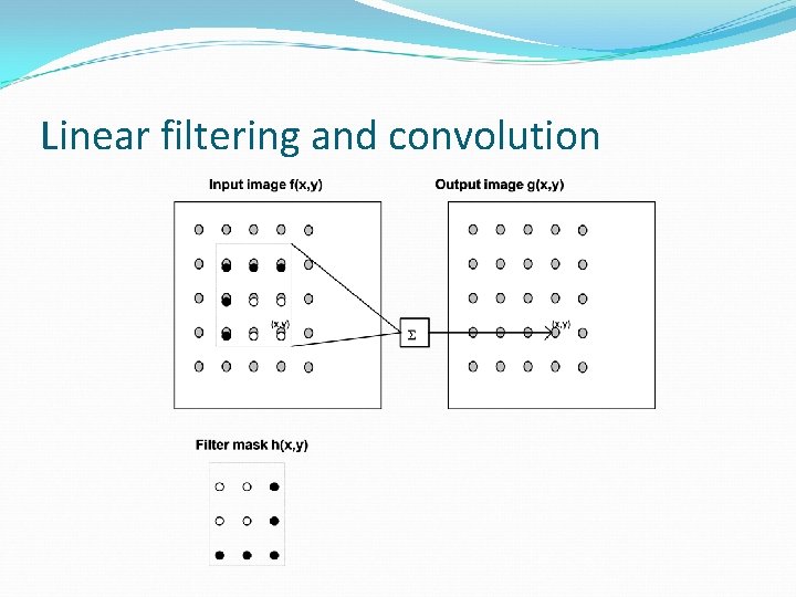
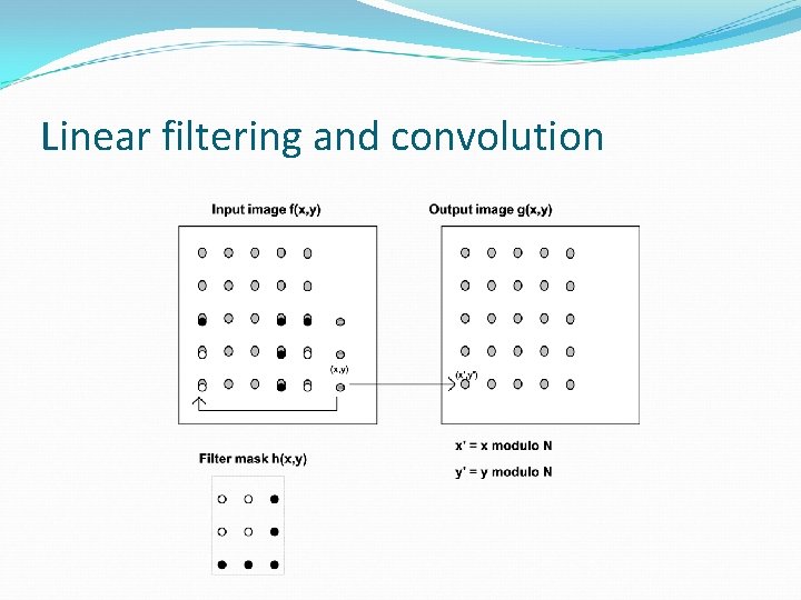
Linear filtering and convolution Convolution involves ‘overlap – multiply – add’ with ‘convolution mask’

Linear filtering and convolution

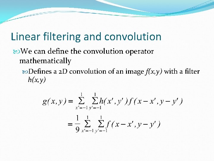
Linear filtering and convolution We can define the convolution operator mathematically Defines a 2 D convolution of an image f(x, y) with a filter h(x, y)

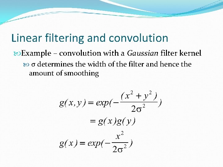
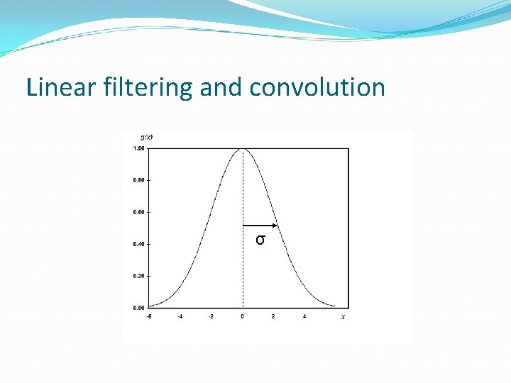
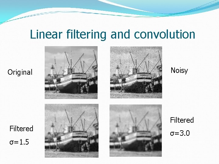
Linear filtering and convolution Example – convolution with a Gaussian filter kernel σ determines the width of the filter and hence the amount of smoothing

Linear filtering and convolution σ

Linear filtering and convolution Original Filtered σ=1. 5 Noisy Filtered σ=3. 0

Linear filtering and convolution Image. J demonstration http: //rsb. info. nih. gov/ij/signed-applet

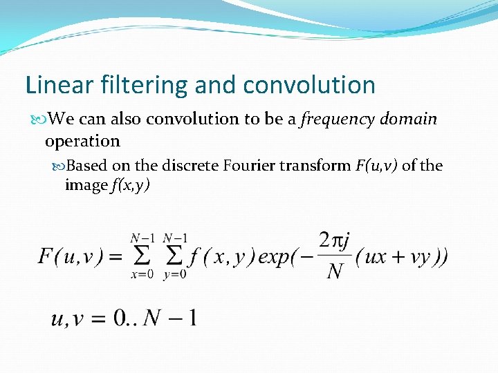
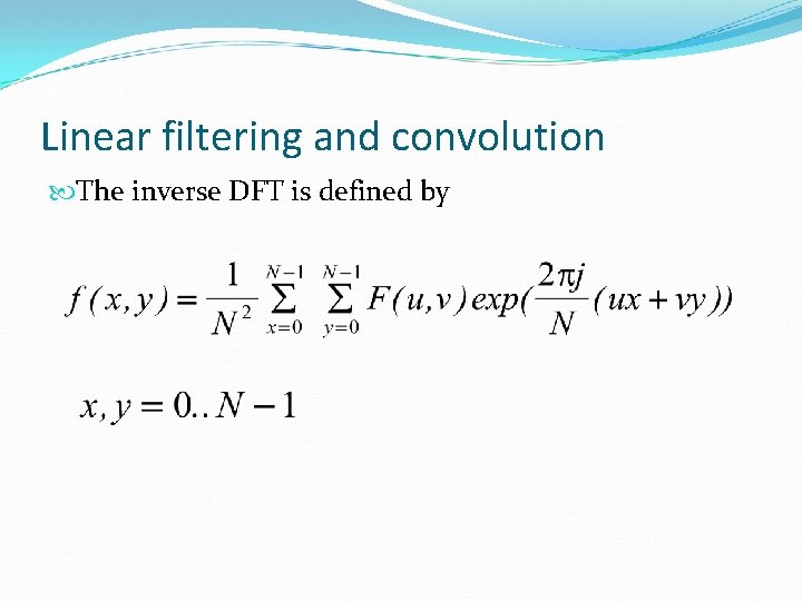
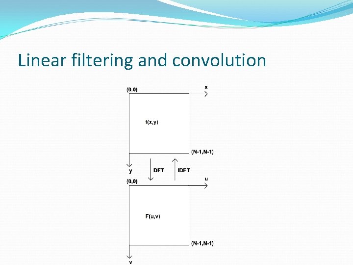
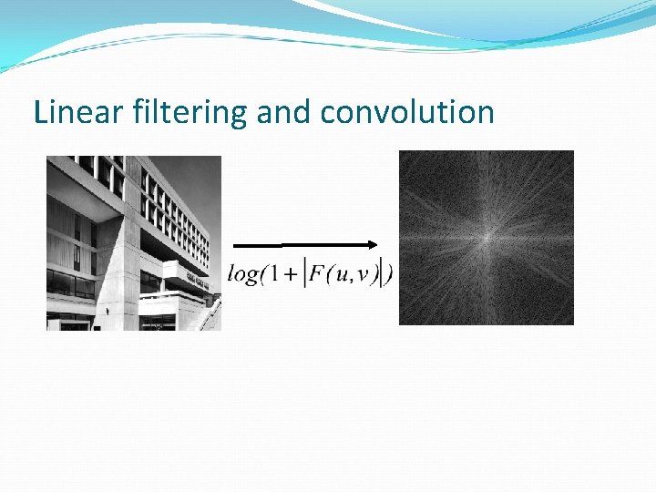
Linear filtering and convolution We can also convolution to be a frequency domain operation Based on the discrete Fourier transform F(u, v) of the image f(x, y)

Linear filtering and convolution The inverse DFT is defined by

Linear filtering and convolution

Linear filtering and convolution

Linear filtering and convolution F(u, v) is the frequency content of the image at spatial frequency position (u, v) Smooth regions of the image contribute low frequency components to F(u, v) Abrupt transitions in grey level (lines and edges) contribute high frequency components to F(u, v)

Linear filtering and convolution We can compute the DFT directly using the formula 2 An N point DFT would require N floating point multiplications per output point 2 Since there are N output points , the computational complexity of the DFT is N 4 4 9 N =4 x 10 for N=256 Bad news! Many hours on a workstation

Linear filtering and convolution The FFT algorithm was developed in the 60’s for seismic exploration 2 Reduced the DFT complexity to 2 N log 2 N 2 6 2 N log 2 N~10 for N=256 A few seconds on a workstation

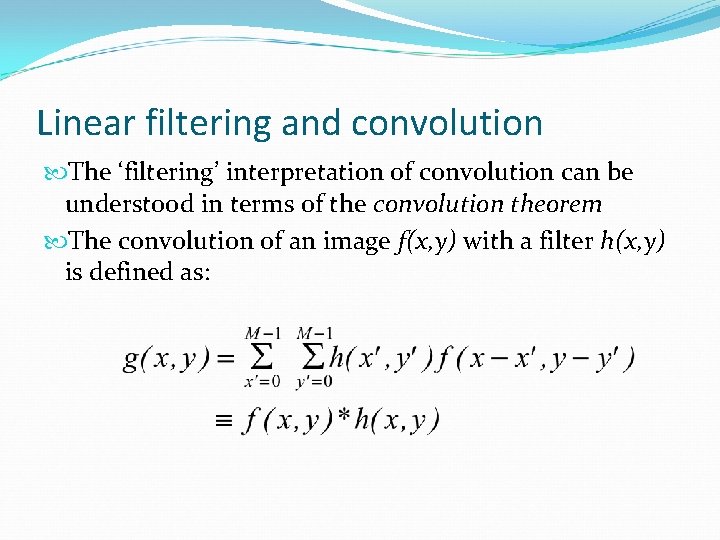
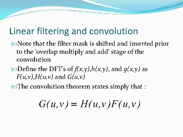
Linear filtering and convolution The ‘filtering’ interpretation of convolution can be understood in terms of the convolution theorem The convolution of an image f(x, y) with a filter h(x, y) is defined as:

Linear filtering and convolution

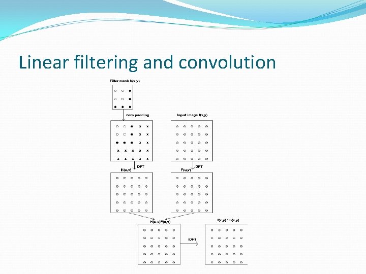
Linear filtering and convolution Note that the filter mask is shifted and inverted prior to the ‘overlap multiply and add’ stage of the convolution Define the DFT’s of f(x, y), h(x, y), and g(x, y) as F(u, v), H(u, v) and G(u, v) The convolution theorem states simply that :

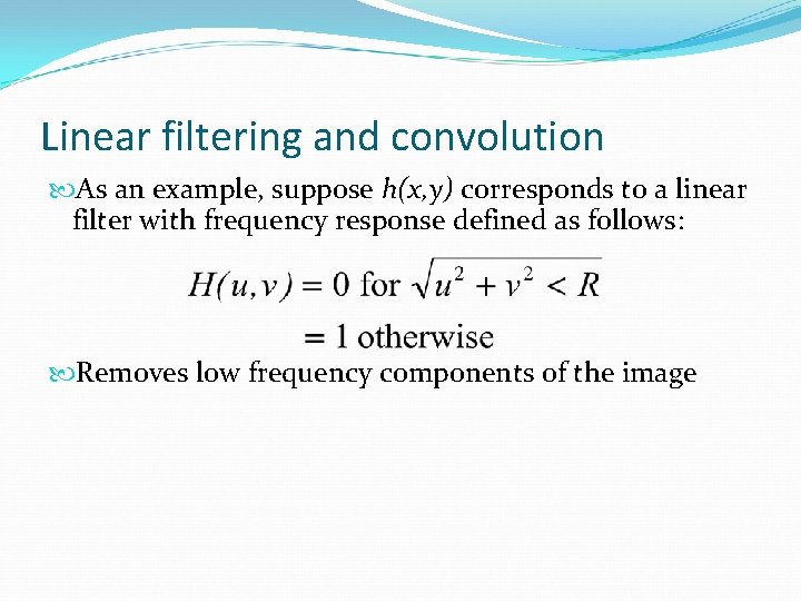
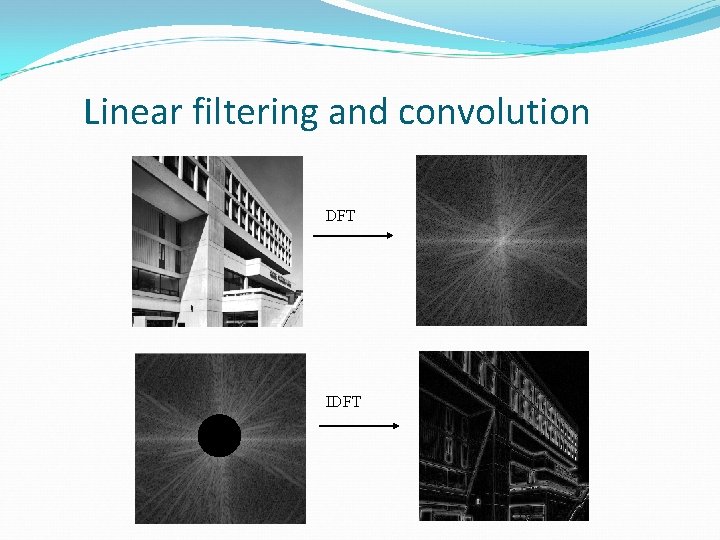
Linear filtering and convolution As an example, suppose h(x, y) corresponds to a linear filter with frequency response defined as follows: Removes low frequency components of the image

Linear filtering and convolution DFT IDFT

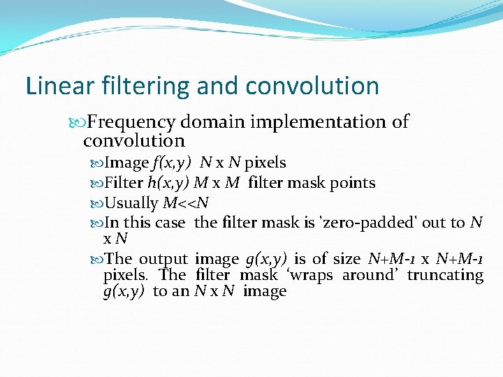
Linear filtering and convolution Frequency domain implementation of convolution Image f(x, y) N x N pixels Filter h(x, y) M x M filter mask points Usually M<<N In this case the filter mask is 'zero-padded' out to N x. N The output image g(x, y) is of size N+M-1 x N+M-1 pixels. The filter mask ‘wraps around’ truncating g(x, y) to an N x N image

Linear filtering and convolution

Linear filtering and convolution

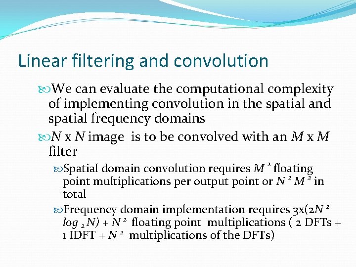
Linear filtering and convolution We can evaluate the computational complexity of implementing convolution in the spatial and spatial frequency domains N x N image is to be convolved with an M x M filter 2 Spatial domain convolution requires M floating point multiplications per output point or N 2 M 2 in total Frequency domain implementation requires 3 x(2 N 2 log 2 N) + N 2 floating point multiplications ( 2 DFTs + 1 IDFT + N 2 multiplications of the DFTs)

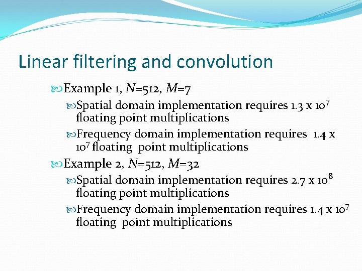
Linear filtering and convolution Example 1, N=512, M=7 Spatial domain implementation requires 1. 3 x 107 floating point multiplications Frequency domain implementation requires 1. 4 x 107 floating point multiplications Example 2, N=512, M=32 Spatial domain implementation requires 2. 7 x 108 floating point multiplications Frequency domain implementation requires 1. 4 x 107 floating point multiplications

Linear filtering and convolution For smaller mask sizes, spatial and frequency domain implementations have about the same computational complexity However, we can speed up frequency domain interpretations by tessellating the image into subblocks and filtering these independently Not quite that simple – we need to overlap the filtered sub-blocks to remove blocking artefacts Overlap and add algorithm

Linear filtering and convolution We can look at some examples of linear filters commonly used in image processing and their frequency responses In particular we will look at a smoothing filter and a filter to perform edge detection

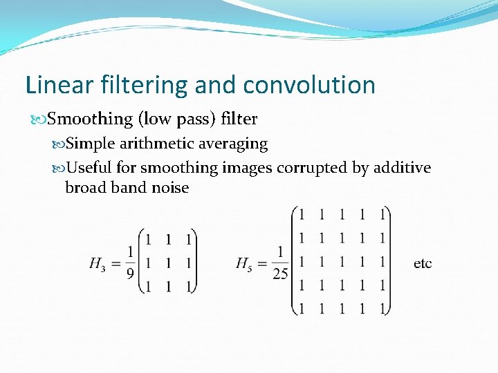
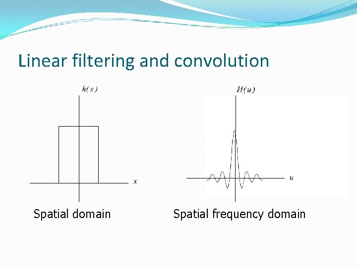
Linear filtering and convolution Smoothing (low pass) filter Simple arithmetic averaging Useful for smoothing images corrupted by additive broad band noise

Linear filtering and convolution Spatial domain Spatial frequency domain

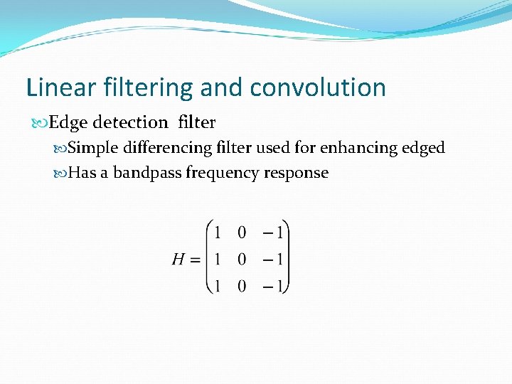
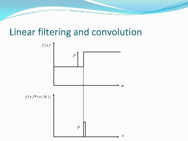
Linear filtering and convolution Edge detection filter Simple differencing filter used for enhancing edged Has a bandpass frequency response

Linear filtering and convolution Image. J demonstration http: //rsb. info. nih. gov/ij/signed-applet

Linear filtering and convolution

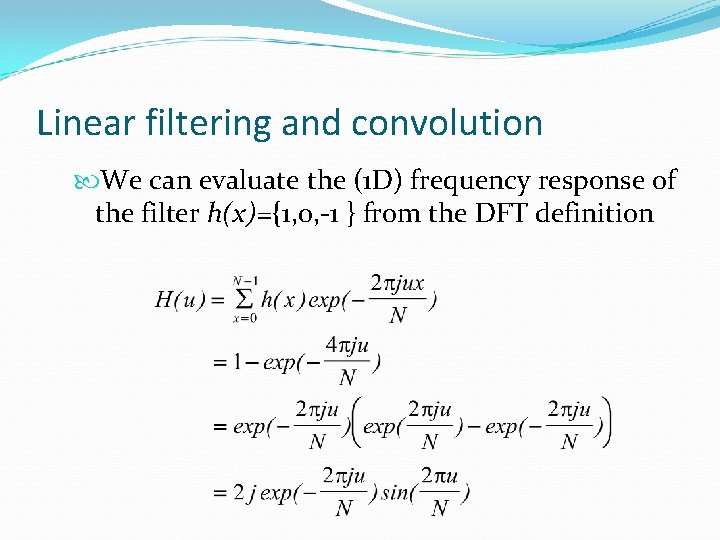
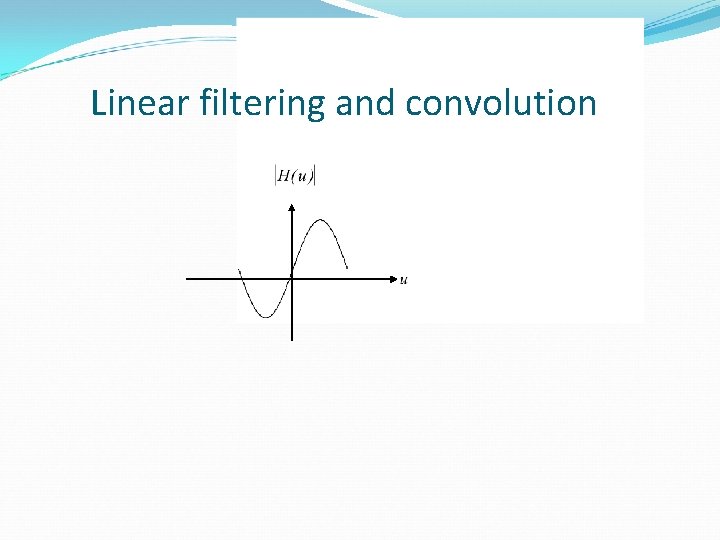
Linear filtering and convolution We can evaluate the (1 D) frequency response of the filter h(x)={1, 0, -1 } from the DFT definition

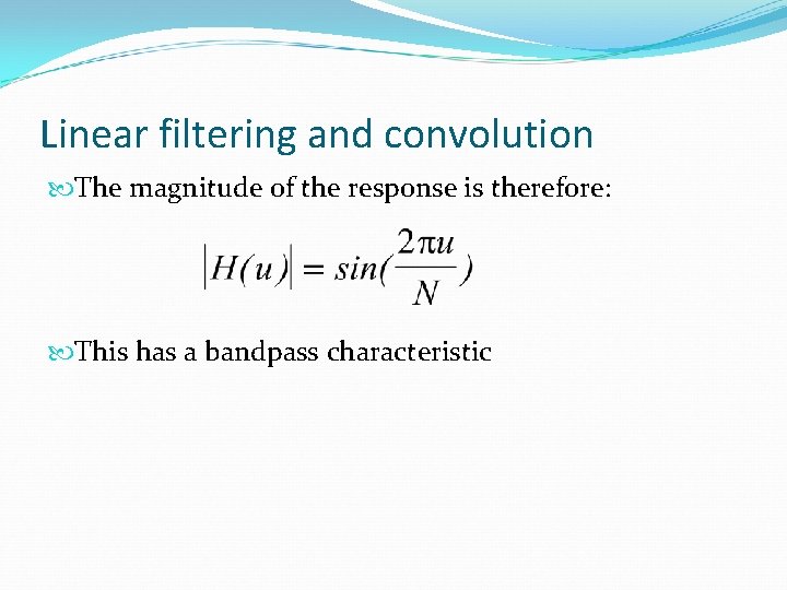
Linear filtering and convolution The magnitude of the response is therefore: This has a bandpass characteristic

Linear filtering and convolution

Conclusion We have looked at basic (low level) image processing operations Enhancement Filtering These are usually important pre-processing steps carried out in computer vision systems (often in hardware)