Image Compression DKLT and DCT Efficient Representation of

Image Compression: DKLT and DCT • Efficient Representation of Signals • Discrete Karhunen-Loeve Transform (DKLT) for 1 D signals • DKLT for 2 D Signals • Discrete Cosine Transform (DCT) for 2 D signals • Application to JPEG

Efficient Representation of Signals Take any audio signal (1 D): most of the times two adjacent values are fairly similar to each other, ie they are correlated. take a small segment: most of the times two adjacent samples have similar values

Efficient Representation of Signals You can see it if you take all pairs of adjacent values (x[2 n] and x[2 n-1]) and plot them as a point in the plane: all distributed along the red axis

Efficient Representation of Signals If we rotate the axis by 45 degrees, we have a more efficient representation, since the second component has a smaller range of values:

Efficient Representation of Signals The effect of this transformation is that it almost decorrelates pairs of samples: Lower Correlation

Efficient Representation of Signals Except for white noise: the samples are already uncorrelated! Plot adjacent values:

Efficient Representation of Signals segment transform quantize encode reconstruct inverse transform decode • The “transform” decorrelates the samples within each segment. Therefore z[n] is a more efficient representation of the signal, since it has less redundant information. • Typical transforms: DKLT, DCT or Wavelets.

Discrete Karhunen-Loeve Transform (DKLT) for 1 D Consider a 1 D signal divide it into segments of length L: L samples

Discrete Karhunen-Loeve Transform (DKLT) for 1 D Signals The goal is to find an L x L matrix Q such that, for all blocks k is such that for denotes expectation and it is meant as average over all the blocks as

Discrete Karhunen-Loeve Transform (DKLT) for 1 D Signals In matrix form this can be formulated as follows: we need to find an L x L matrix Q such that with From the definition: where blocks. is the L x L autocorrelation of the signal

Discrete Karhunen-Loeve Transform (DKLT) for 1 D Signals In order to find two matrices Q and recall eigenvalues and eigenvectors of Define then and (diagonal) such that as

Discrete Karhunen-Loeve Transform (DKLT) for 1 D Signals Since the autocorrelation matrix is hermitian (ie positive semidefinite, they have the following properties: and real for Therefore: Eigenvectors and Eigenvalues of ) and

Discrete Karhunen-Loeve Transform (DKLT) for 1 D Signals The autocorrelation matrix is computed as with

Discrete Karhunen-Loeve Transform (DKLT) for 1 D Signals Example: 1 D Signal. Choose segment length L=64 samples:

Discrete Karhunen-Loeve Transform (DKLT) for 1 D Signals Compute 64 x 64 autocorrelation matrix: rxx=xcorr(x)/length(x); Rxx=fftshift(rxx); Rxx=toeplitz(rxx(1: 64)); [Q, Lambda]=eig(Rxx)

Discrete Karhunen-Loeve Transform (DKLT) for 1 D Signals 64 eigenvectors close to sinusoids! 64 eigenvalues Notice: only a few dominant eigenvalues

Discrete Karhunen-Loeve Transform (DKLT) for 1 D Signals Compare one section with its own transform: a few dominant values all small values

Discrete Karhunen-Loeve Transform (DKLT) for 1 D Signals The autocorrelation matrix is a toeplitz matrix, associated to the correlation sequence and it is defined as

Discrete Karhunen-Loeve Transform (DKLT) for 1 D Signals Notice: same values over each diagonal. Example: In matlab: R= C= Rxx=toeplitz(C, R);

DKLT for 2 D Signals Same for 2 D. We can divide the image into non overlapping blocks of size. Reshape into a vector:

DKLT for 2 D Signals In 2 D: Block Toeplitz with

DKLT for 2 D Signals Each block which is Toeplitz. is given by

DKLT for 2 D Signals Then the autocorrelation matrix is . In this case L=3:

DKLT for 2 D Signals In Matlab we use xcorr 2. If the image “x” is Nx. N, then is an N-1 x. N-1 matrix, with the “zero lag” at index (N, N), as Then, for L=3: column row

Example of DKLT eigenvalues 8 x 8 eigenvectors

Example of DKLT 8 x 8 eigenvectors eigenvalues

Discrete Cosine Transform (DCT) for 2 D Signals Fact: the eigenvectors of the autocorrelation matrix are very close to sinusoidal. This is due to the particular Toeplitz structure of the autocorrelation matrix. Therefore if we use sinusoids as basis signals, we obtain a close approximation to the DKLT, with the advantages that a) the basis signals are not data dependent, so we do not have to send them; b) the DCT is very efficient in terms of computation (very close to the FFT).

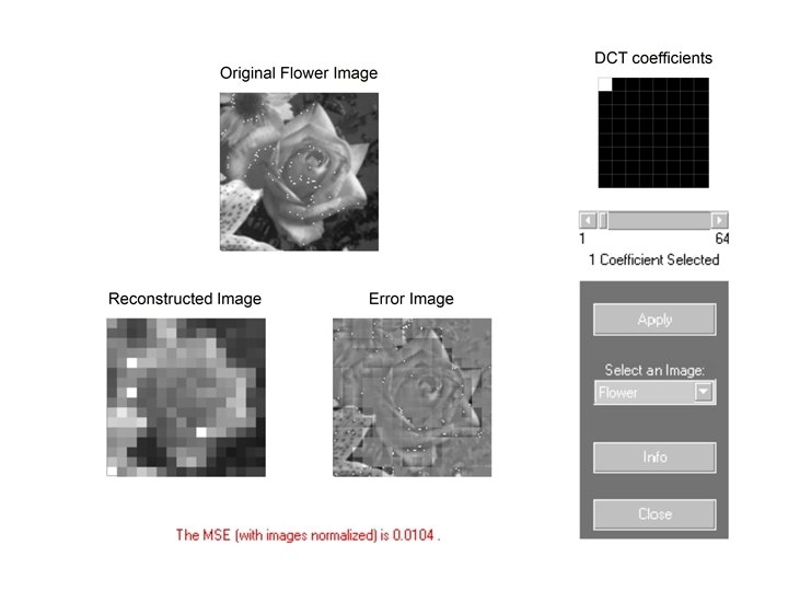
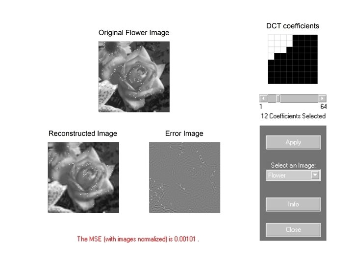
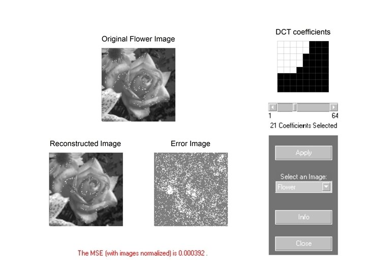
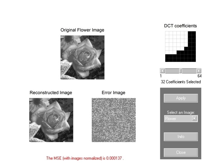
Discrete Cosine Transform (DCT) for 2 D Signals Each 8 x 8 block is expanded in terms of 64 basis functions, which are 2 D cosines with

Discrete Cosine Transform (DCT) for 2 D Signals Basis Signals

Discrete Cosine Transform (DCT) for 2 D Signals Problem: represent the image data with the fewest number of data points. Divide the Image into blocks (usually 8 x 8 or 16 x 16 pixels) Low Frequencies DCT Middle Frequencies High Frequencies