
Image and Video Processing III 3 10 Basic
Image and Video Processing
III. 3. 10 Basic Methods for Motion Detection • 1 Introduction • 2 Frame Difference – 2. 1 Scale filter – 2. 2 Three-frame difference – 2. 3 Accumulative difference picture • 3 Background Subtraction – 3. 1 Simple background modeling – 3. 2 GMM based background subtraction • 4 Optical Flow Field – 4. 1 Horn-Schunck algorithm – 4. 2 Lucas-Kanade algorithm
1. Introduction • What is motion detection? -Whether image points are moving or not? • Motion detection is the process of detecting a change in the position of an object relative to its surroundings or a change in the surroundings relative to an object. • What’s the reason for motion detection? • In motion analysis, the main task of motion detection is to detect moving targets. It lays the foundation for subsequent motion feature extraction and recognition. • What are the basic methods? • Frame difference, Background subtraction, Optical flow field.
Motion Detection Goals of motion detection • Identify moving objects • Detection of unusual activity patterns • Computing trajectories of moving objects Applications of motion detection • Indoor/outdoor security • Real time crime detection • Traffic monitoring Many intelligent video analysis systems are based on motion detection.
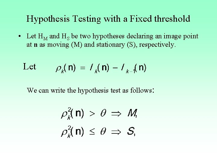
Hypothesis Testing with a Fixed threshold • Let HM and HS be two hypotheses declaring an image point at n as moving (M) and stationary (S), respectively. Let We can write the hypothesis test as follows :
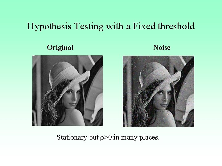
Hypothesis Testing with a Fixed threshold Original Noise Stationary but ρ>θ in many places.
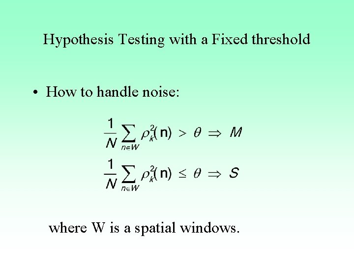
Hypothesis Testing with a Fixed threshold • How to handle noise: where W is a spatial windows.
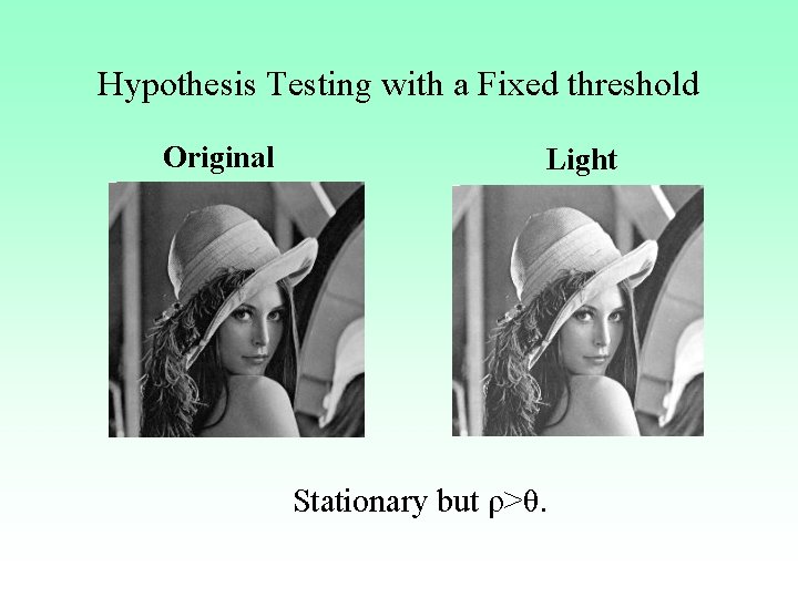
Hypothesis Testing with a Fixed threshold Original Light Stationary but ρ>θ.
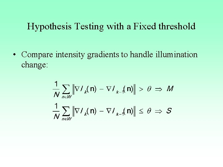
Hypothesis Testing with a Fixed threshold • Compare intensity gradients to handle illumination change:
III. 2 Basic Methods for Motion Detection • 1 Introduction • 2 Frame Difference – 2. 1 Scale filter – 2. 2 Three-frame difference – 2. 3 Accumulative difference picture • 3 Background Subtraction – 3. 1 Simple background modeling – 3. 2 GMM based background subtraction • 4 Optical Flow Field – 4. 1 Horn-Schunck algorithm – 4. 2 Lucas-Kanade algorithm
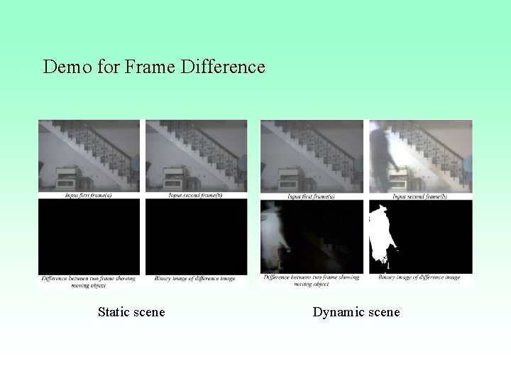
Demo for Frame Difference Static scene Dynamic scene
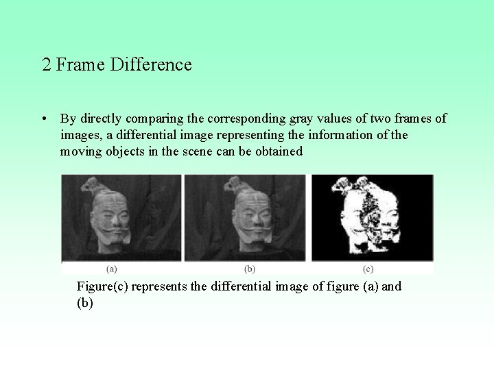
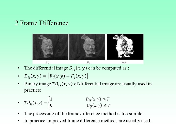
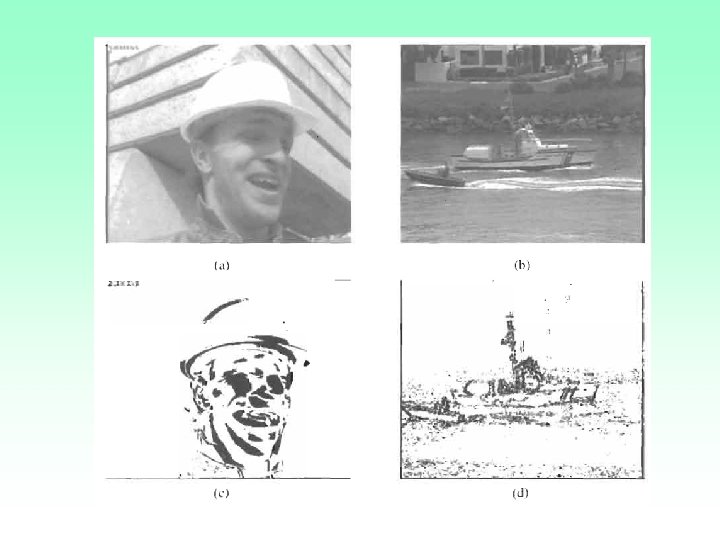
2 Frame Difference • By directly comparing the corresponding gray values of two frames of images, a differential image representing the information of the moving objects in the scene can be obtained Figure(c) represents the differential image of figure (a) and (b)
2 Frame Difference •
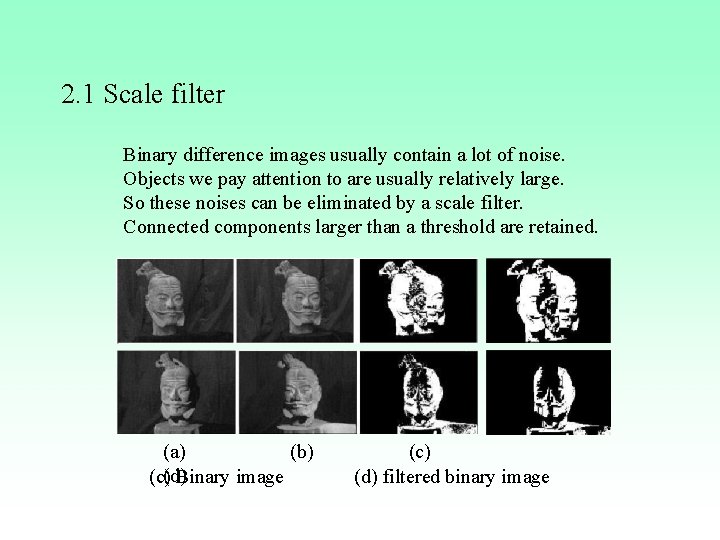
2. 1 Scale filter Binary difference images usually contain a lot of noise. Objects we pay attention to are usually relatively large. So these noises can be eliminated by a scale filter. Connected components larger than a threshold are retained. (a) (b) (c) (d) (c) Binary image (d) filtered binary image
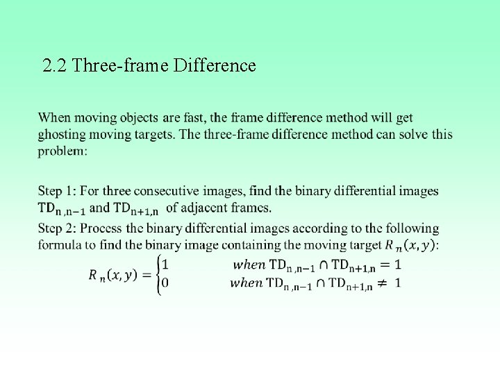
2. 2 Three-frame Difference •
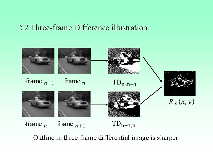
2. 2 Three-frame Difference illustration Outline in three-frame differential image is sharper.
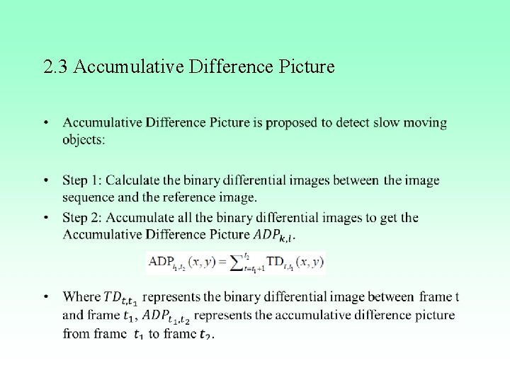
2. 3 Accumulative Difference Picture •
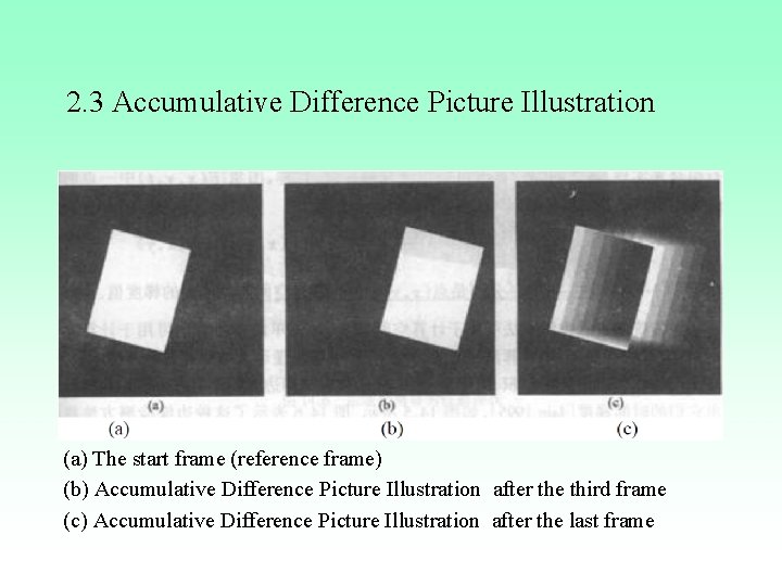
2. 3 Accumulative Difference Picture Illustration (a) The start frame (reference frame) (b) Accumulative Difference Picture Illustration after the third frame (c) Accumulative Difference Picture Illustration after the last frame
III. 2 Basic Methods for Motion Detection • 1 Introduction • 2 Frame Difference – 2. 1 Scale filter – 2. 2 Three-frame difference – 2. 3 Accumulative difference picture • 3 Background Subtraction – 3. 1 Simple background modeling – 3. 2 GMM based background subtraction • 4 Optical Flow Field – 4. 1 Horn-Schunck algorithm – 4. 2 Lucas-Kanade algorithm
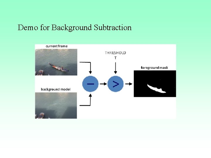
Demo for Background Subtraction
3 Background Subtraction • Background subtraction aims to detect moving objects from the video (image) sequence and reduce the background • It can simplify various video image processing problems, reduce the amount of calculation and model complexity. • The basic process of background subtraction is: • Step 1: Modeling the background • Step 2: Calculating the binary differential image between frame and background
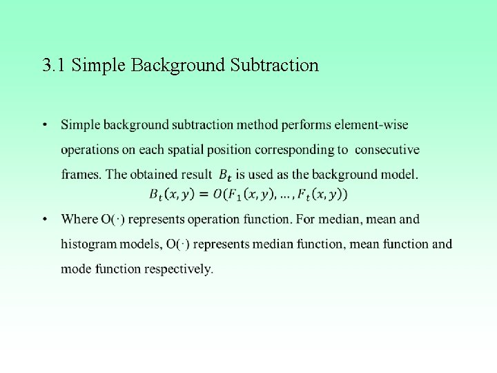
3. 1 Simple Background Subtraction •
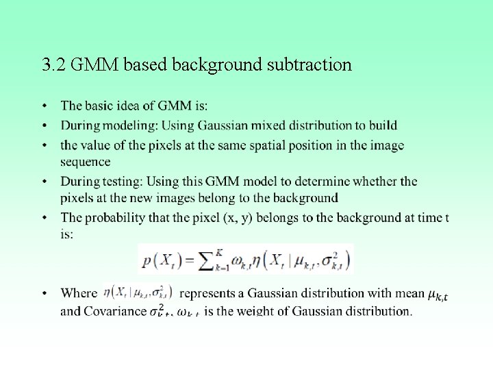
3. 2 GMM based background subtraction •
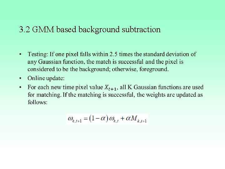
3. 2 GMM based background subtraction •
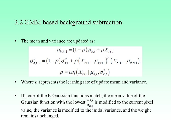
3. 2 GMM based background subtraction •
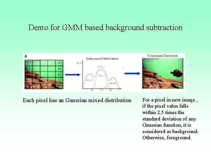
Demo for GMM based background subtraction Each pixel has an Gaussian mixed distribution For a pixel in new image , if the pixel value falls within 2. 5 times the standard deviation of any Gaussian function, it is considered as background. Otherwise, foreground.
III. 2 Basic Methods for Motion Detection • 1 Introduction • 2 Frame Difference – 2. 1 Scale filter – 2. 2 Three-frame difference – 2. 3 Accumulative difference picture • 3 Background Subtraction – 3. 1 Simple background modeling – 3. 2 GMM based background subtraction • 4 Optical Flow Field – 4. 1 Horn-Schunck algorithm – 4. 2 Lucas-Kanade algorithm
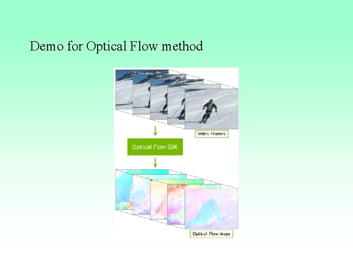
Demo for Optical Flow method
4 Optical Flow Field • Optical flow is the pattern of apparent motion of objects, surfaces and edges in a visual scene caused by the relative motion between an observer and a scene. • Optical flow can also be defined as the distribution of apparent velocities of movement of brightness pattern in an image. • By detecting the change of the brightness of the pixel of the image over time, we can calculate optical flow.
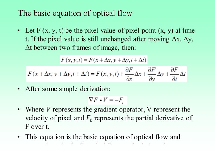
The basic equation of optical flow •
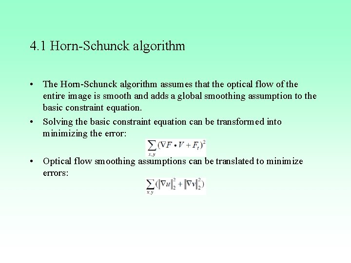
4. 1 Horn-Schunck algorithm • The Horn-Schunck algorithm assumes that the optical flow of the entire image is smooth and adds a global smoothing assumption to the basic constraint equation. • Solving the basic constraint equation can be transformed into minimizing the error: • Optical flow smoothing assumptions can be translated to minimize errors:
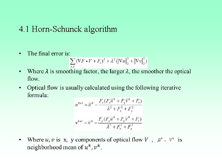
4. 1 Horn-Schunck algorithm •
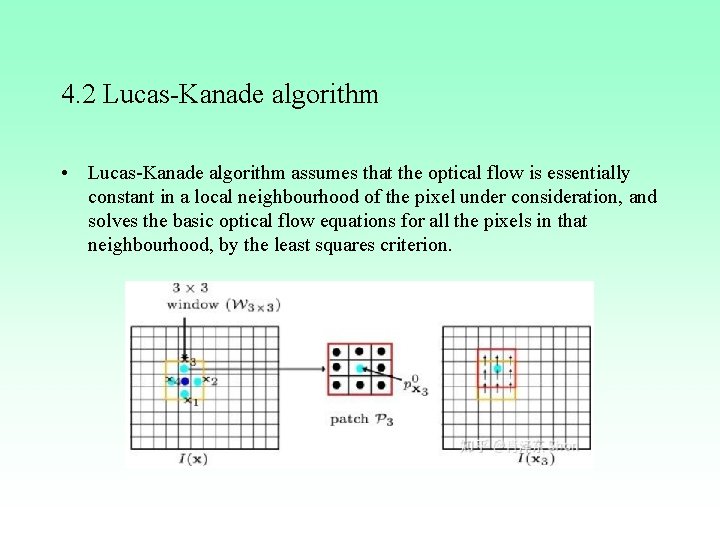
4. 2 Lucas-Kanade algorithm • Lucas-Kanade algorithm assumes that the optical flow is essentially constant in a local neighbourhood of the pixel under consideration, and solves the basic optical flow equations for all the pixels in that neighbourhood, by the least squares criterion.
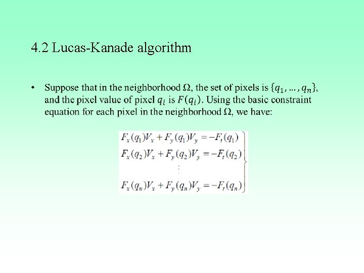
4. 2 Lucas-Kanade algorithm •
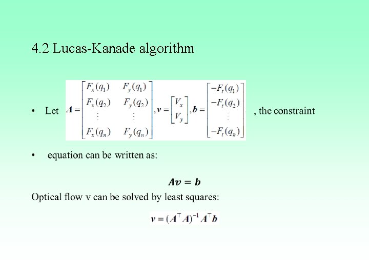
4. 2 Lucas-Kanade algorithm •
Motion Estimation
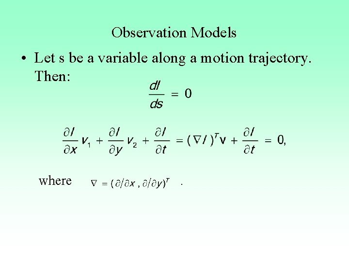
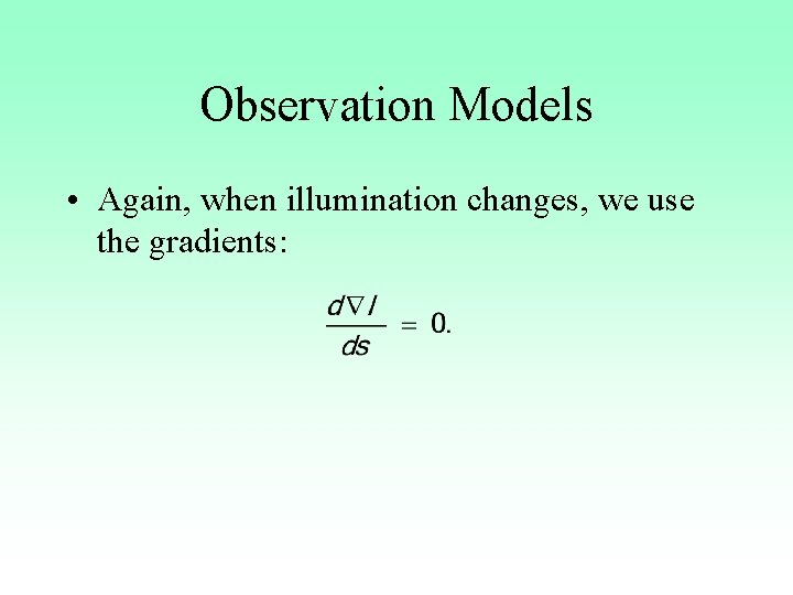
Motion Models • • Spatial Motion Models Temporal Motion Models Region of Support Observation Models
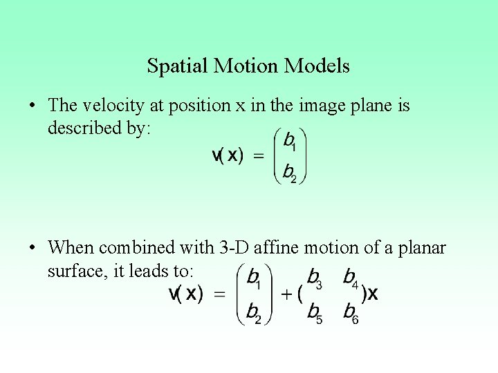
Spatial Motion Models • The velocity at position x in the image plane is described by: • When combined with 3 -D affine motion of a planar surface, it leads to:
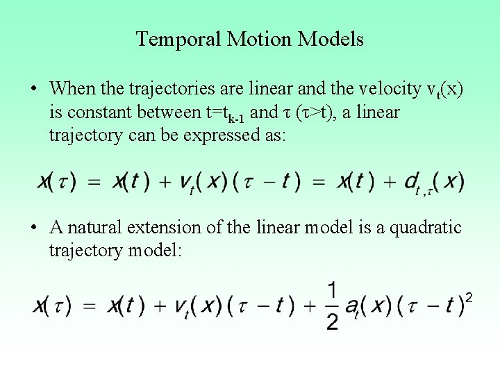
Temporal Motion Models • When the trajectories are linear and the velocity vt(x) is constant between t=tk-1 and τ (τ>t), a linear trajectory can be expressed as: • A natural extension of the linear model is a quadratic trajectory model:
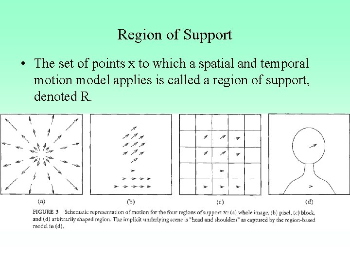
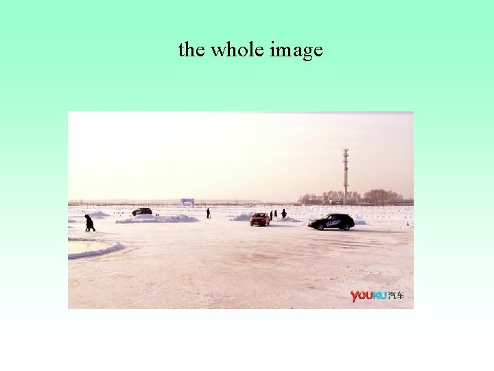
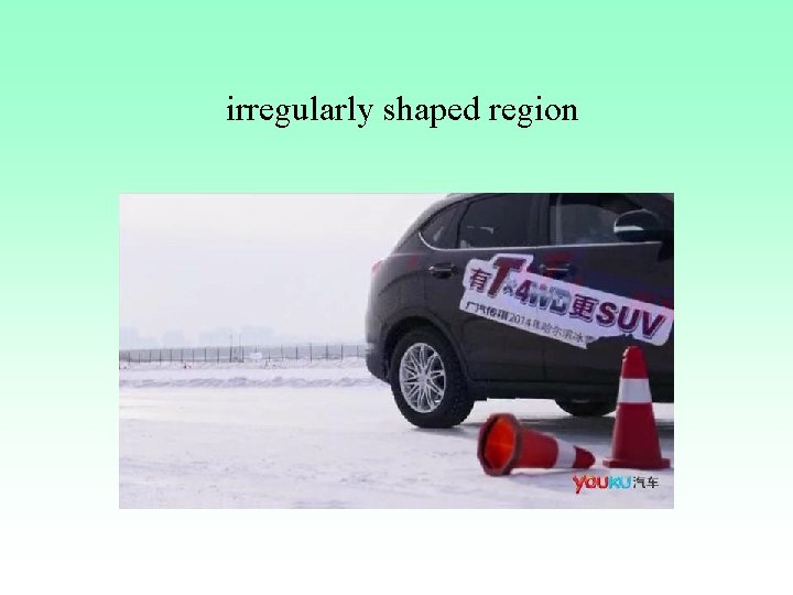
Region of Support • The set of points x to which a spatial and temporal motion model applies is called a region of support, denoted R.
the whole image
irregularly shaped region
Observation Models • Let s be a variable along a motion trajectory. Then: where .
Observation Models • Again, when illumination changes, we use the gradients:
Estimation Criteria The models discussed have to be incorporated into an estimation criterion that will be subsequently optimized. • Pixel-Domain Criteria • Regularization • Bayesian Criteria
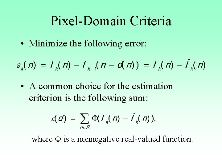
Pixel-Domain Criteria • Minimize the following error: • A common choice for the estimation criterion is the following sum: where Φ is a nonnegative real-valued function.
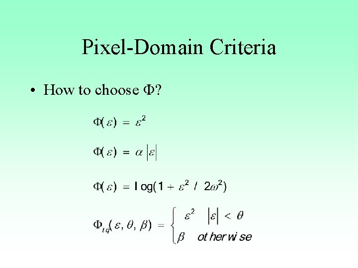
Pixel-Domain Criteria • How to choose Φ?
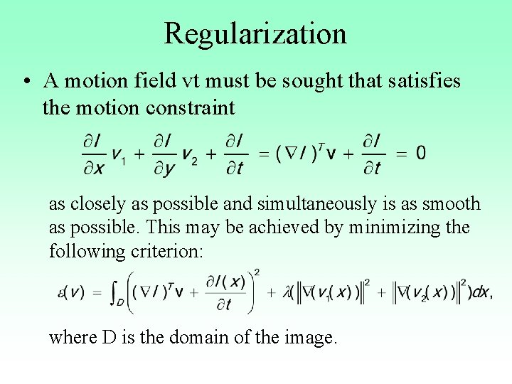
Regularization • A motion field vt must be sought that satisfies the motion constraint as closely as possible and simultaneously is as smooth as possible. This may be achieved by minimizing the following criterion: where D is the domain of the image.
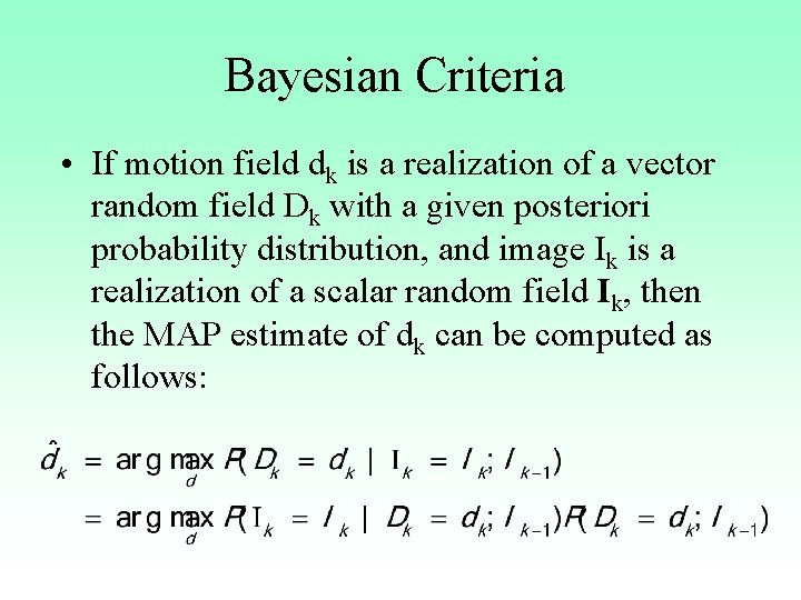
Bayesian Criteria • If motion field dk is a realization of a vector random field Dk with a given posteriori probability distribution, and image Ik is a realization of a scalar random field Ik, then the MAP estimate of dk can be computed as follows:
Search Strategies • Once models have been identified and incorporated into an estimation criterion, the last step is to develop an efficient (complexity) and effective (solution quality) strategy for finding the estimates of motion parameters. – Minimizing a prediction error – Gradient-based techniques – Relaxation techniques
Practical Motion Estimation Algorithms • • • Global Motion Estimation Block Matching Phase Correlation Optical Flow by Means of Regularization MAP Estimation of Dense Motion
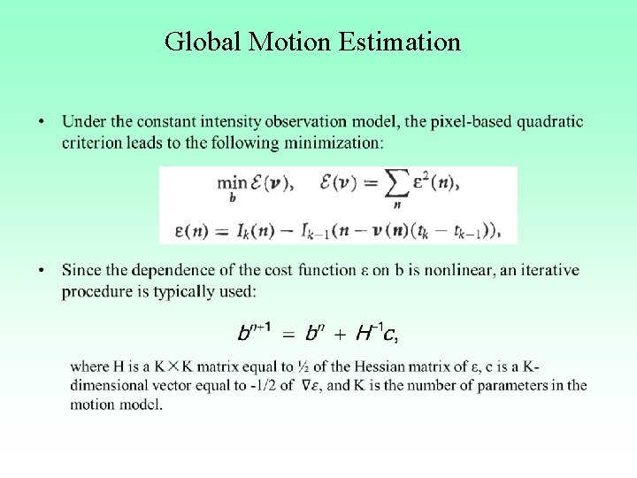
Global Motion Estimation •
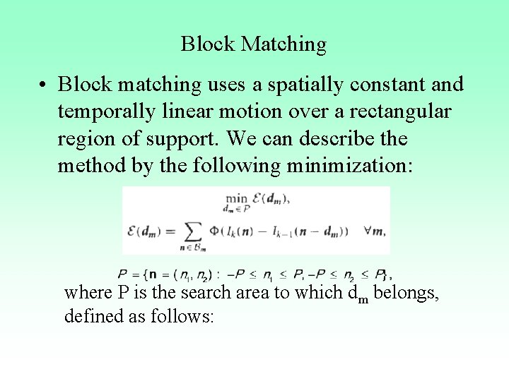
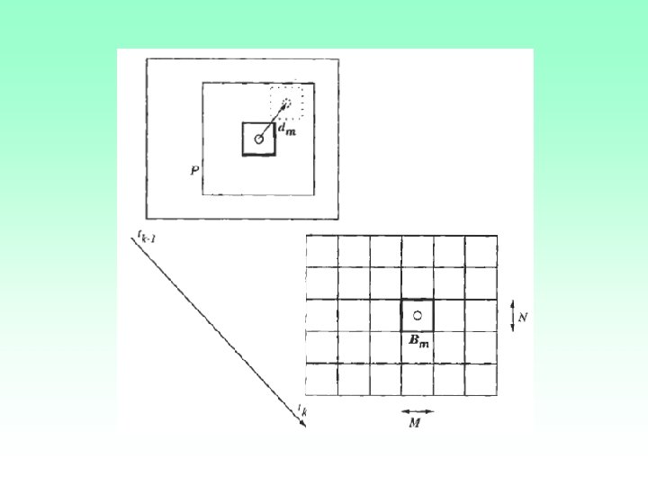
Block Matching • Block matching uses a spatially constant and temporally linear motion over a rectangular region of support. We can describe the method by the following minimization: where P is the search area to which dm belongs, defined as follows:
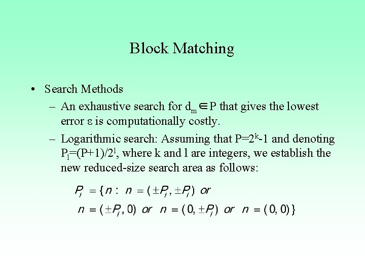
Block Matching • Search Methods – An exhaustive search for dm∈P that gives the lowest error ε is computationally costly. – Logarithmic search: Assuming that P=2 k-1 and denoting Pl=(P+1)/2 l, where k and l are integers, we establish the new reduced-size search area as follows:
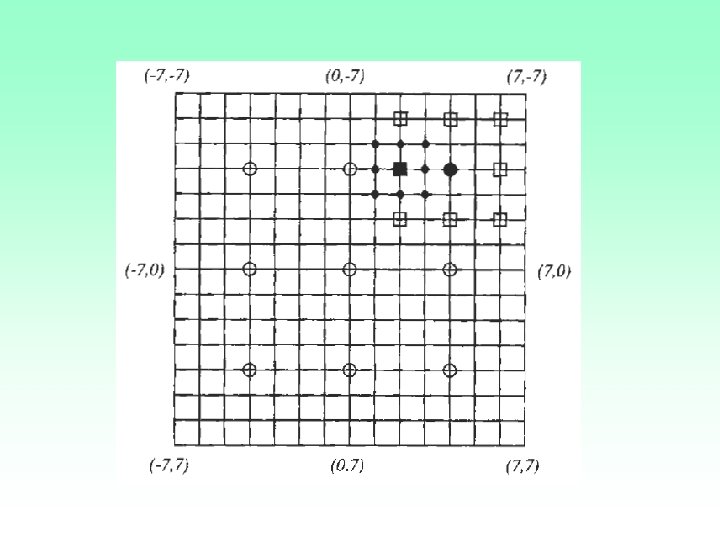
Block Matching • 2 -D search vs 1 -D search – One-at-a-time search – Parallel hierarchical one-dimensional search – ……
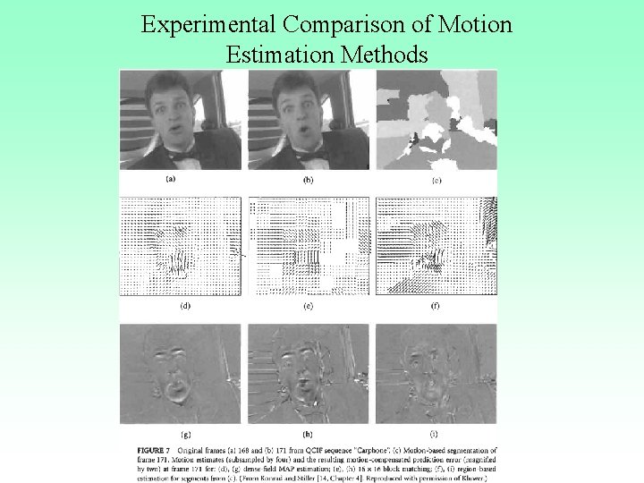
Experimental Comparison of Motion Estimation Methods
- Slides: 59