Image and Video Coding and Processing Lecture 5

Image (and Video) Coding and Processing Lecture 5: Point Operations Wade Trappe

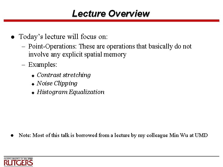
Lecture Overview l Today’s lecture will focus on: – Point-Operations: These are operations that basically do not involve any explicit spatial memory – Examples: u u u l Contrast stretching Noise Clipping Histogram Equalization Note: Most of this talk is borrowed from a lecture by my colleague Min Wu at UMD

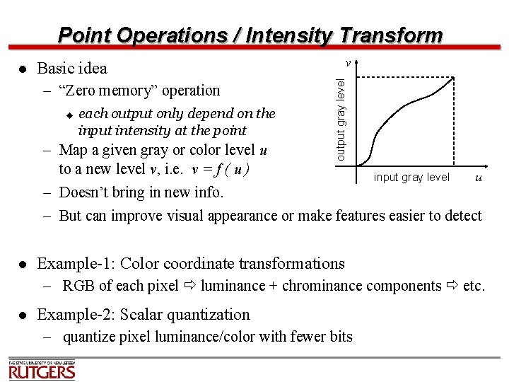
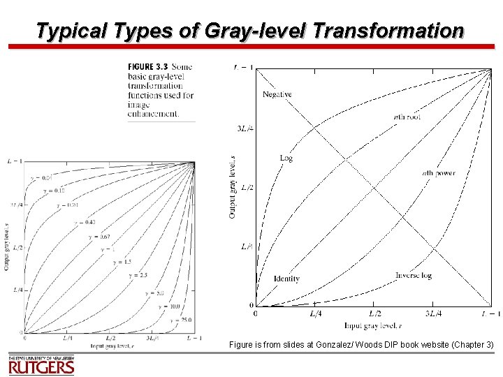
Point Operations / Intensity Transform v Basic idea – “Zero memory” operation u each output only depend on the input intensity at the point output gray level l – Map a given gray or color level u to a new level v, i. e. v = f ( u ) input gray level u – Doesn’t bring in new info. – But can improve visual appearance or make features easier to detect l Example-1: Color coordinate transformations – RGB of each pixel luminance + chrominance components etc. l Example-2: Scalar quantization – quantize pixel luminance/color with fewer bits

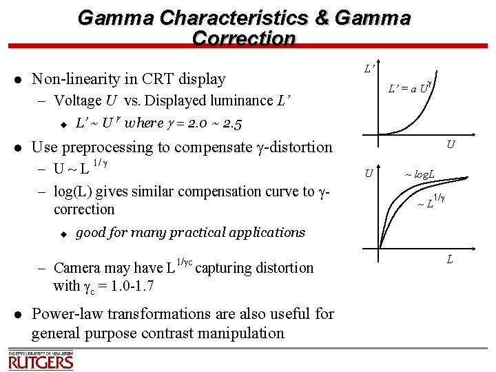
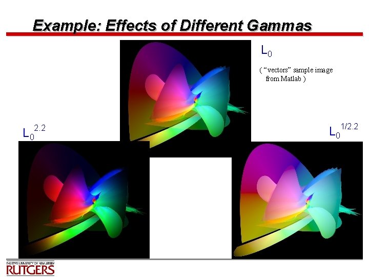
Gamma Characteristics & Gamma Correction l Non-linearity in CRT display L’ L’ = a U – Voltage U vs. Displayed luminance L’ u l L’ ~ U where = 2. 0 ~ 2. 5 Use preprocessing to compensate -distortion – U ~ L 1/ – log(L) gives similar compensation curve to correction u U U ~ log. L ~L 1/ good for many practical applications – Camera may have L 1/ c capturing distortion with c = 1. 0 -1. 7 l Power-law transformations are also useful for general purpose contrast manipulation L

Typical Types of Gray-level Transformation Figure is from slides at Gonzalez/ Woods DIP book website (Chapter 3)

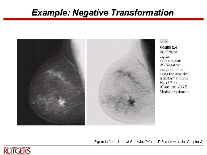
Example: Negative Transformation Figure is from slides at Gonzalez/ Woods DIP book website (Chapter 3)

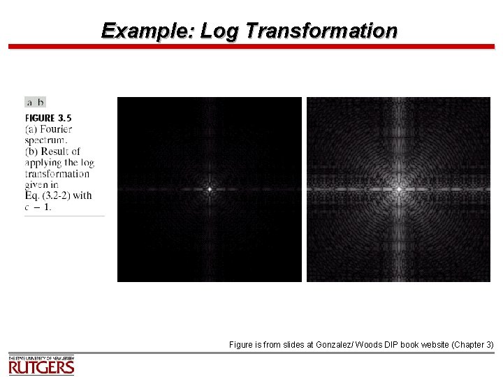
Example: Log Transformation Figure is from slides at Gonzalez/ Woods DIP book website (Chapter 3)

Example: Effects of Different Gammas L 0 ( “vectors” sample image from Matlab ) L 0 2. 2 L 0 1/2. 2

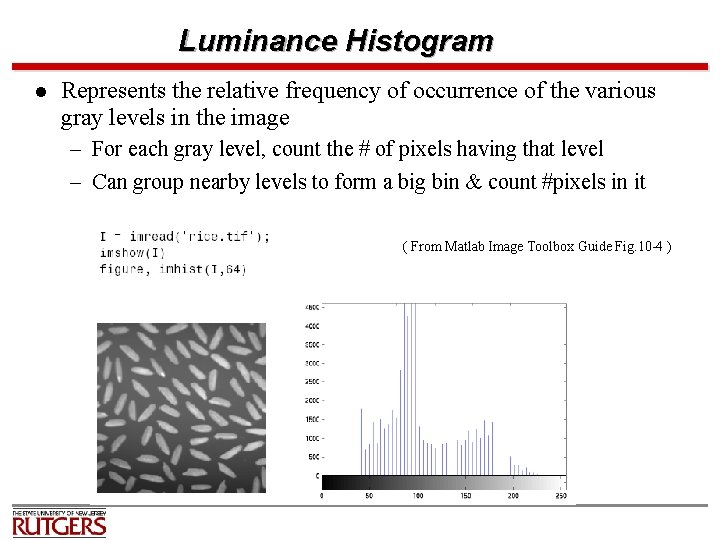
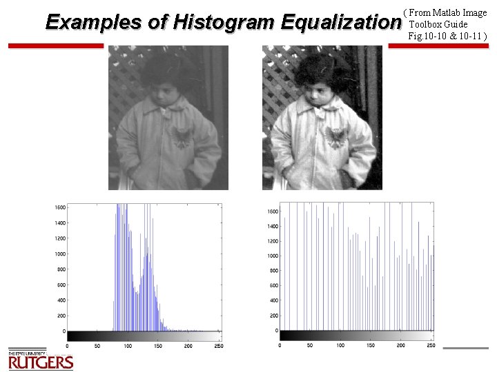
Luminance Histogram l Represents the relative frequency of occurrence of the various gray levels in the image – For each gray level, count the # of pixels having that level – Can group nearby levels to form a big bin & count #pixels in it ( From Matlab Image Toolbox Guide Fig. 10 -4 )

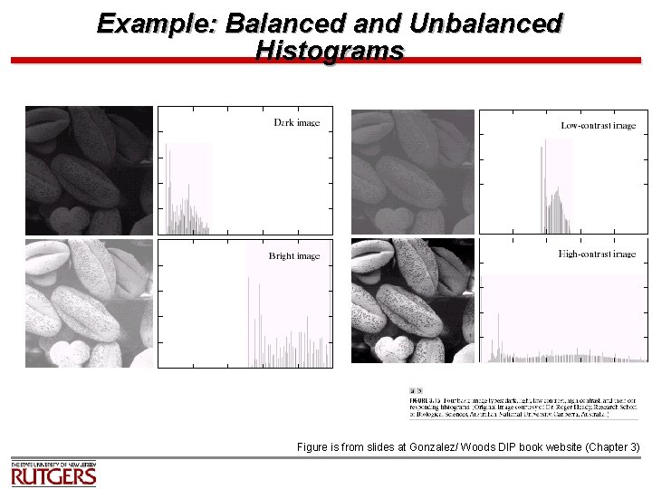
Luminance Histogram (cont’d) l Interpretation – Treat pixel values as i. i. d random variables – Histogram is an estimate of the probability distribution of the r. v. l “Unbalanced” histogram doesn’t fully utilize the dynamic range – Low contrast image ~ histogram concentrating in a narrow luminance range – Under-exposed image ~ histogram concentrating on the dark side – Over-exposed image ~ histogram concentrating on the bright side l Balanced histogram gives more pleasant look and reveals rich content

Example: Balanced and Unbalanced Histograms Figure is from slides at Gonzalez/ Woods DIP book website (Chapter 3)

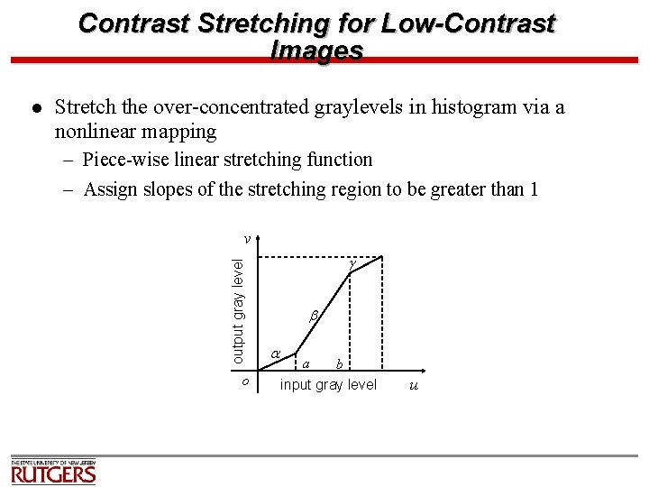
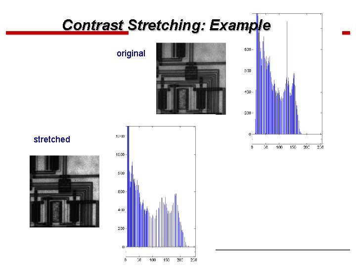
Contrast Stretching for Low-Contrast Images Stretch the over-concentrated graylevels in histogram via a nonlinear mapping – Piece-wise linear stretching function – Assign slopes of the stretching region to be greater than 1 v output gray level l o a b input gray level u

Contrast Stretching: Example original stretched

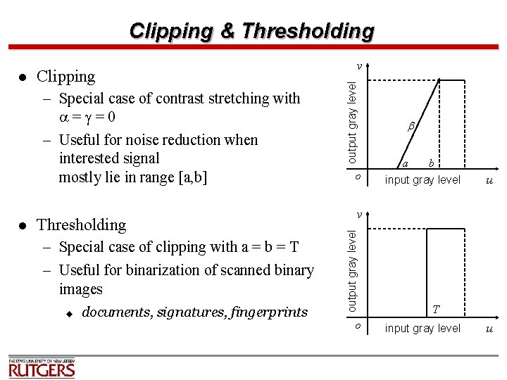
Clipping & Thresholding – Special case of contrast stretching with = =0 – Useful for noise reduction when interested signal mostly lie in range [a, b] l Thresholding – Special case of clipping with a = b = T – Useful for binarization of scanned binary images u documents, signatures, fingerprints output gray level Clipping o a b input gray level u v output gray level l v o T input gray level u

Examples of Histogram Equalization ( From Matlab Image Toolbox Guide Fig. 10 -10 & 10 -11 )

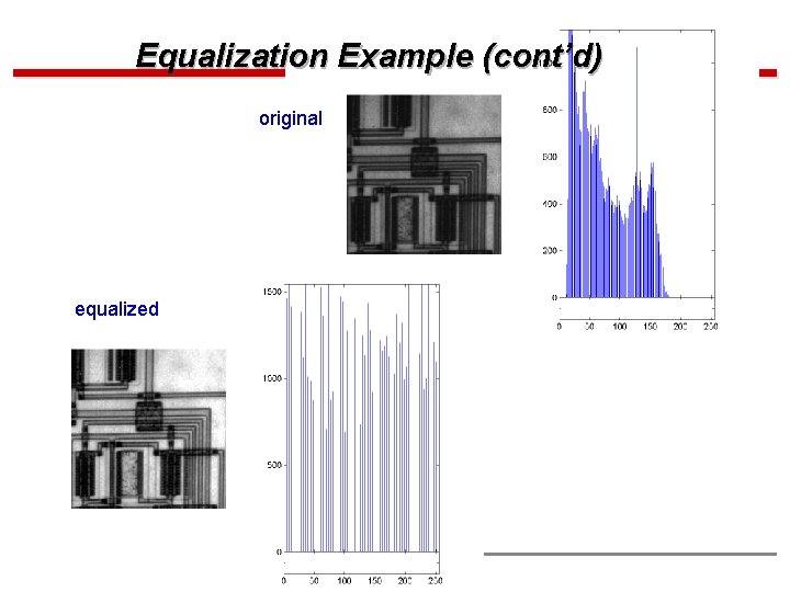
Equalization Example (cont’d) original equalized

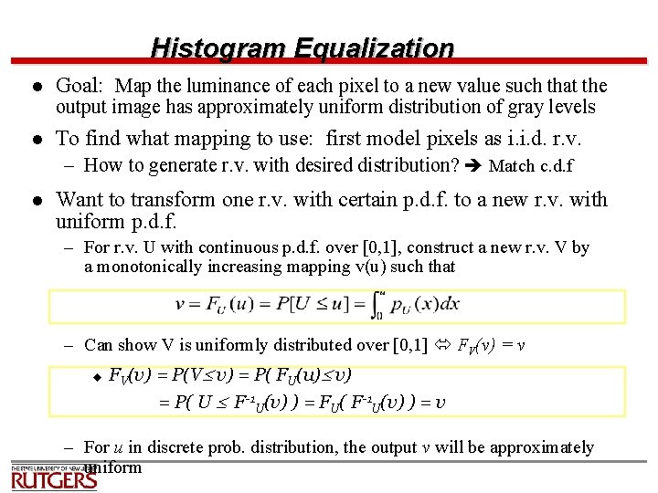
Histogram Equalization l Goal: Map the luminance of each pixel to a new value such that the l To find what mapping to use: first model pixels as i. i. d. r. v. output image has approximately uniform distribution of gray levels – How to generate r. v. with desired distribution? Match c. d. f l Want to transform one r. v. with certain p. d. f. to a new r. v. with uniform p. d. f. – For r. v. U with continuous p. d. f. over [0, 1], construct a new r. v. V by a monotonically increasing mapping v(u) such that – Can show V is uniformly distributed over [0, 1] FV(v) = v u FV(v) = P(V v) = P( FU(u) v) = P( U F-1 U(v) ) = FU( F-1 U(v) ) = v – For u in discrete prob. distribution, the output v will be approximately uniform

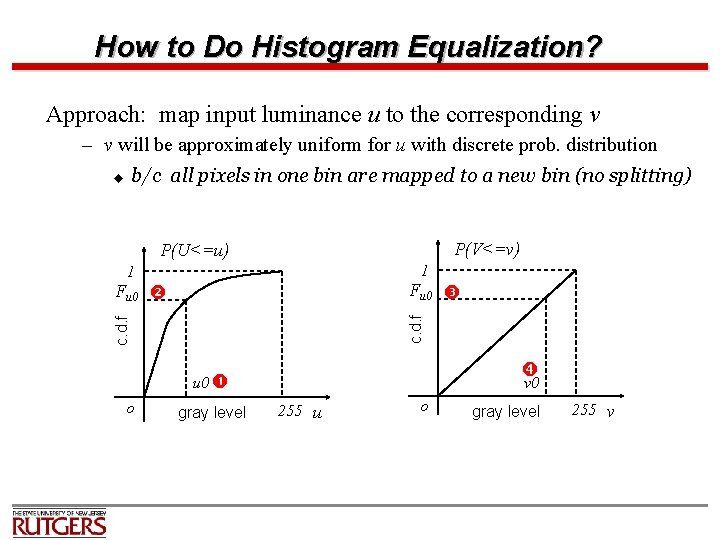
How to Do Histogram Equalization? Approach: map input luminance u to the corresponding v – v will be approximately uniform for u with discrete prob. distribution b/c all pixels in one bin are mapped to a new bin (no splitting) u P(V<=v) P(U<=u) 1 1 Fu 0 c. d. f Fu 0 o gray level v 0 255 u o gray level 255 v

Histogram Equalization Algorithm u v Uniform quantization v’ p. U(xi) v [0, 1] • Map discrete v [0, 1] to v’ {0, …, L-1} • vmin is the smallest positive value of v • vmin 0 1 L-1

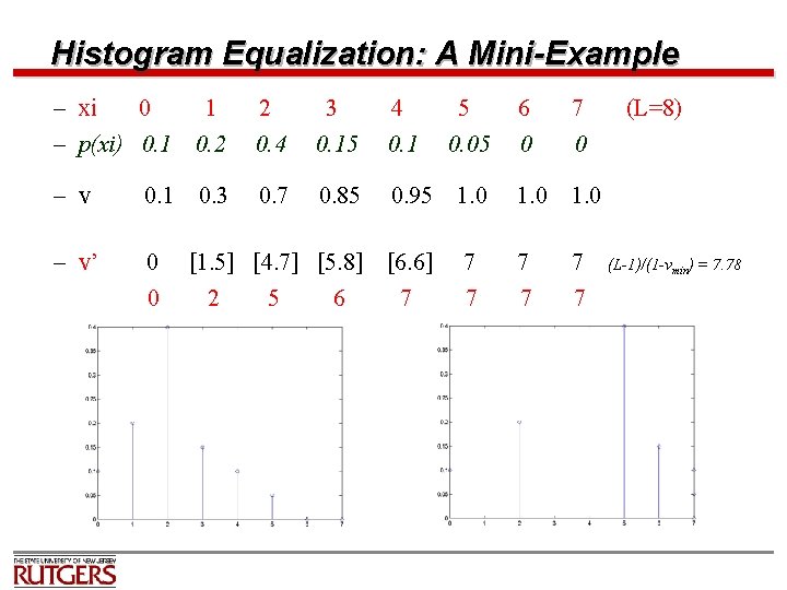
Histogram Equalization: A Mini-Example – xi 0 1 – p(xi) 0. 1 0. 2 2 0. 4 3 0. 15 4 0. 1 – v 0. 1 0. 7 0. 85 – v’ 0 0 [1. 5] [4. 7] [5. 8] 2 5 6 0. 3 5 0. 05 6 0 7 0 0. 95 1. 0 [6. 6] 7 7 7 7 (L=8) (L-1)/(1 -vmin) = 7. 78

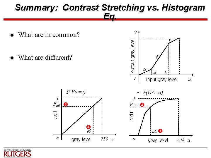
Summary: Contrast Stretching vs. Histogram Eq. What are in common? l What are different? v output gray level l o P(V<=v) b input gray level u P(U<=u) 1 1 Fu 0 c. d. f Fu 0 v 0 o a gray level 255 v o gray level 255 u

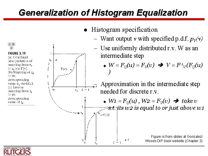
Generalization of Histogram Equalization l Histogram specification – Want output v with specified p. d. f. p. V(v) – Use uniformly distributed r. v. W as an intermediate step u W = FU(u) = FV(v) V = F-1 V (FU(u) ) – Approximation in the intermediate step needed for discrete r. v. u W 1 = FU(u) , W 2 = FV(v) take v s. t. its w 2 is equal to or just above w 1 Figure is from slides at Gonzalez/ Woods DIP book website (Chapter 3)

For Next Time… l Next time we will focus on quantization