Image and Video Coding and Processing Lecture 2

Image (and Video) Coding and Processing Lecture 2: Basic Filtering Wade Trappe

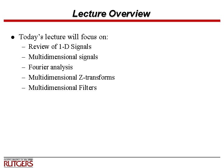
Lecture Overview l Today’s lecture will focus on: – – – Review of 1 -D Signals Multidimensional signals Fourier analysis Multidimensional Z-transforms Multidimensional Filters

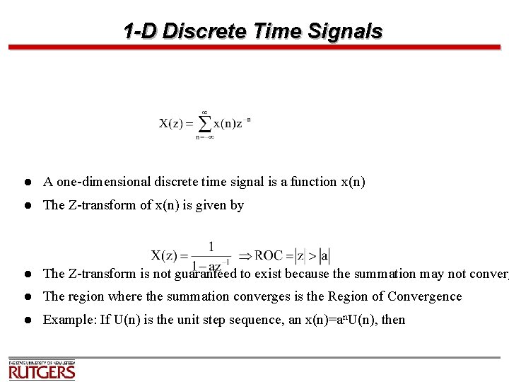
1 -D Discrete Time Signals l A one-dimensional discrete time signal is a function x(n) l The Z-transform of x(n) is given by l The Z-transform is not guaranteed to exist because the summation may not converg l The region where the summation converges is the Region of Convergence l Example: If U(n) is the unit step sequence, an x(n)=an. U(n), then

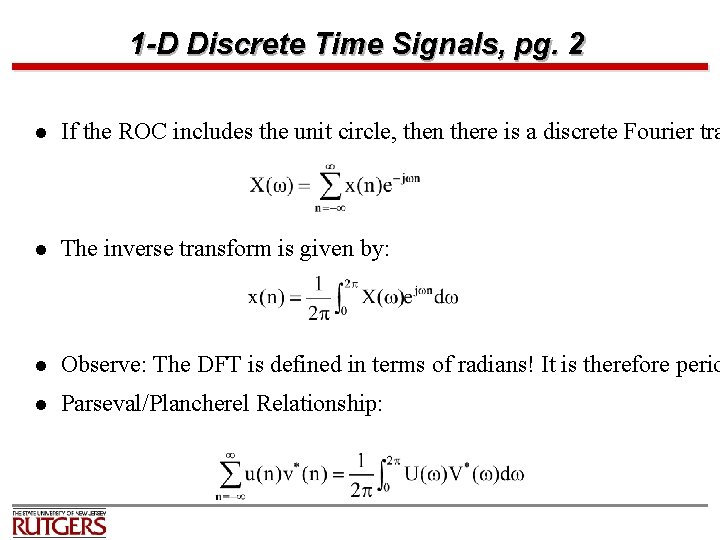
1 -D Discrete Time Signals, pg. 2 l If the ROC includes the unit circle, then there is a discrete Fourier tra l The inverse transform is given by: l Observe: The DFT is defined in terms of radians! It is therefore perio l Parseval/Plancherel Relationship:

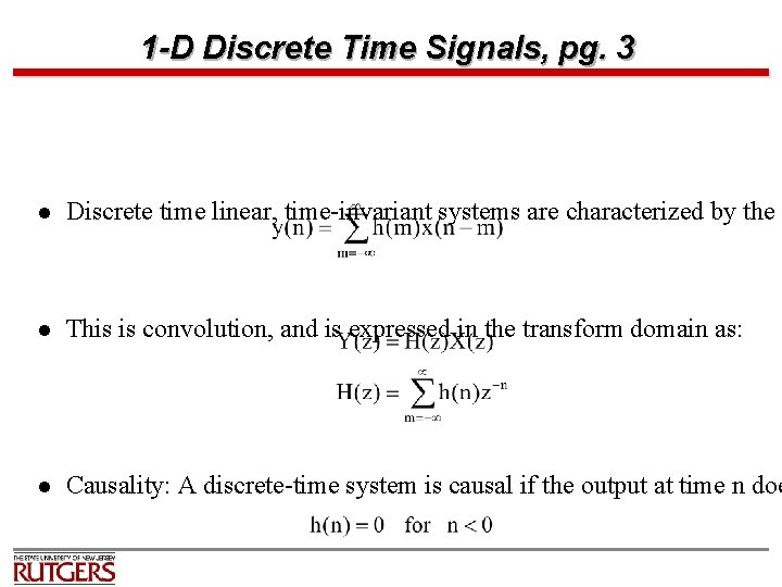
1 -D Discrete Time Signals, pg. 3 l Discrete time linear, time-invariant systems are characterized by the i l This is convolution, and is expressed in the transform domain as: l Causality: A discrete-time system is causal if the output at time n doe

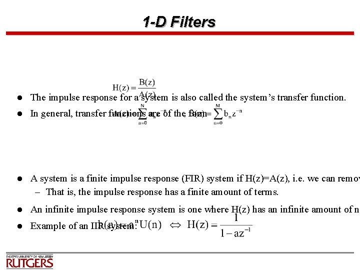
1 -D Filters l The impulse response for a system is also called the system’s transfer function. l In general, transfer functions are of the form l A system is a finite impulse response (FIR) system if H(z)=A(z), i. e. we can remov – That is, the impulse response has a finite amount of terms. l An infinite impulse response system is one where H(z) has an infinite amount of no l Example of an IIR system:

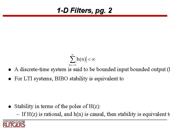
1 -D Filters, pg. 2 l A discrete-time system is said to be bounded input bounded output (B l For LTI systems, BIBO stability is equivalent to l Stability in terms of the poles of H(z): – If H(z) is rational, and h(n) is causal, then stability is equivalent to

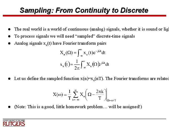
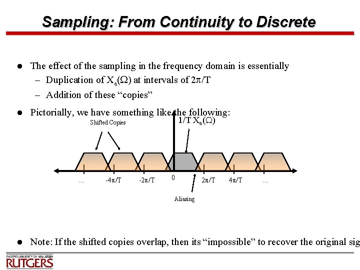
Sampling: From Continuity to Discrete l The real world is a world of continuous (analog) signals, whether it is sound or ligh To process signals we will need “sampled” discrete-time signals Analog signals xa(t) have Fourier transform pairs l Let us define the sampled function x(n)=xa(n. T). The Fourier transforms are related l (Note: This is a good, little homework problem… will be assigned!) l l

Sampling: From Continuity to Discrete l The effect of the sampling in the frequency domain is essentially – Duplication of Xa(W) at intervals of 2 p/T – Addition of these “copies” l Pictorially, we have something like the following: 1/T Xa(W) Shifted Copies … -4 p/T -2 p/T 0 2 p/T 4 p/T … Aliasing l Note: If the shifted copies overlap, then its “impossible” to recover the original sig

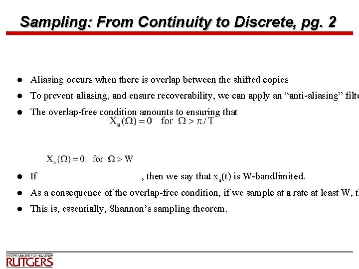
Sampling: From Continuity to Discrete, pg. 2 l Aliasing occurs when there is overlap between the shifted copies l To prevent aliasing, and ensure recoverability, we can apply an “anti-aliasing” filte l The overlap-free condition amounts to ensuring that l If l As a consequence of the overlap-free condition, if we sample at a rate at least W, th l This is, essentially, Shannon’s sampling theorem. , then we say that xa(t) is W-bandlimited.

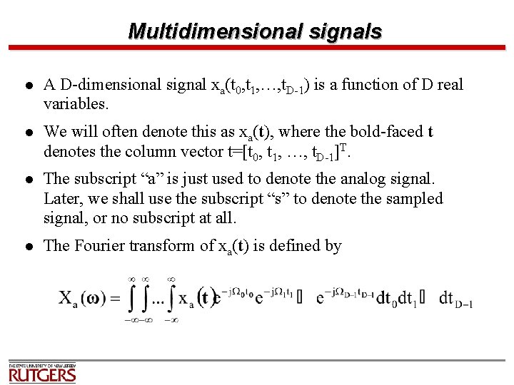
Multidimensional signals l A D-dimensional signal xa(t 0, t 1, …, t. D-1) is a function of D real variables. l We will often denote this as xa(t), where the bold-faced t denotes the column vector t=[t 0, t 1, …, t. D-1]T. l The subscript “a” is just used to denote the analog signal. Later, we shall use the subscript “s” to denote the sampled signal, or no subscript at all. l The Fourier transform of xa(t) is defined by

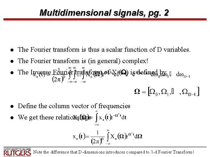
Multidimensional signals, pg. 2 l The Fourier transform is thus a scalar function of D variables. l The Fourier transform is (in general) complex! l The Inverse Fourier transform of Xa(W) is defined by l Define the column vector of frequencies l We get these relationships Note the difference that D-dimensions introduces compared to 1 -d Fourier Transform!

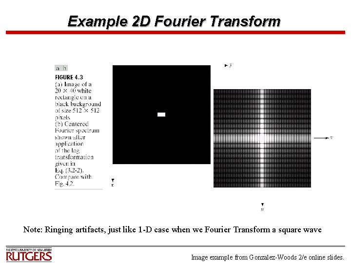
Example 2 D Fourier Transform Note: Ringing artifacts, just like 1 -D case when we Fourier Transform a square wave Image example from Gonzalez-Woods 2/e online slides.

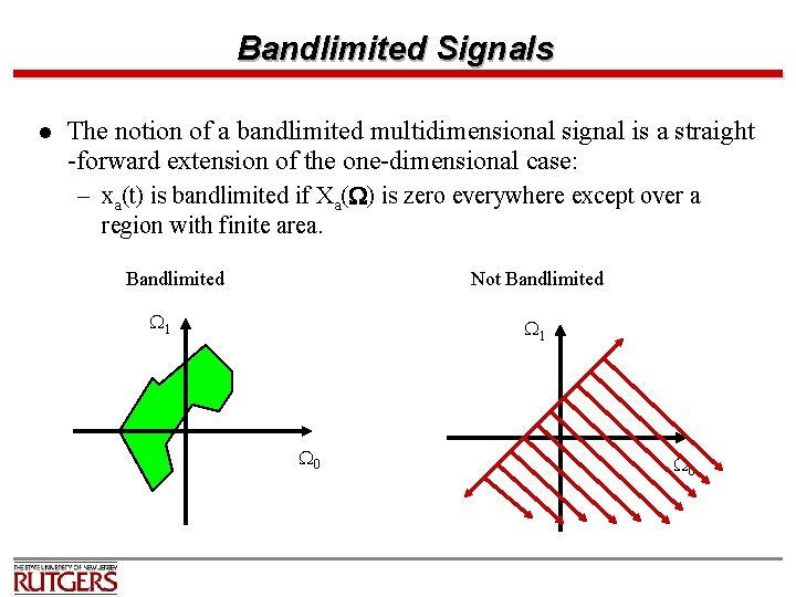
Bandlimited Signals l The notion of a bandlimited multidimensional signal is a straight -forward extension of the one-dimensional case: – xa(t) is bandlimited if Xa(W) is zero everywhere except over a region with finite area. Bandlimited Not Bandlimited W 1 W 0

Multidimensional Sampled Signals l We will use n=[n 0, n 1, …, n. D-1]T to denote an arbitrary Ddimensional vector of integer values l A signal x(n) is just a function of D integer values l The Fourier transform of x(n) and the inverse transform are given by l Key point: X(w) is periodic in each variable wi with period 2 p

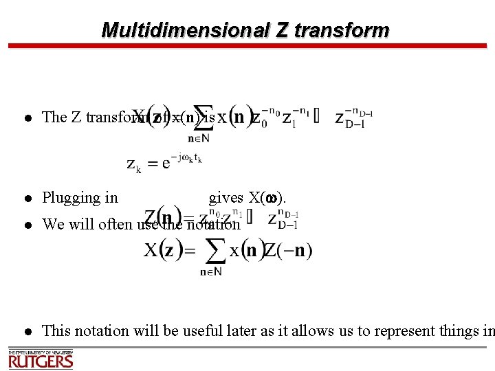
Multidimensional Z transform l The Z transform of x(n) is l Plugging in l We will often use the notation l This notation will be useful later as it allows us to represent things in gives X(w).

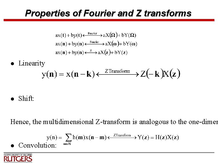
Properties of Fourier and Z transforms l Linearity l Shift: Hence, the multidimensional Z-transform is analogous to the one-dimen l Convolution:

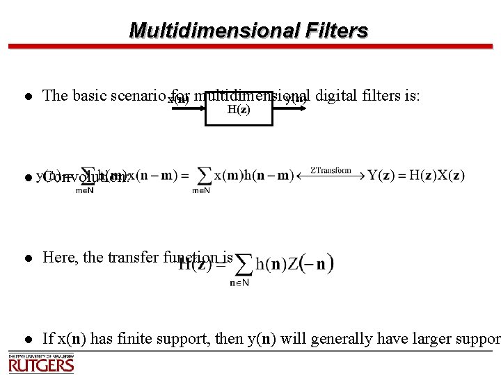
Multidimensional Filters l The basic scenario x(n) for multidimensional y(n) digital filters is: l Convolution: l Here, the transfer function is l If x(n) has finite support, then y(n) will generally have larger suppor H(z)

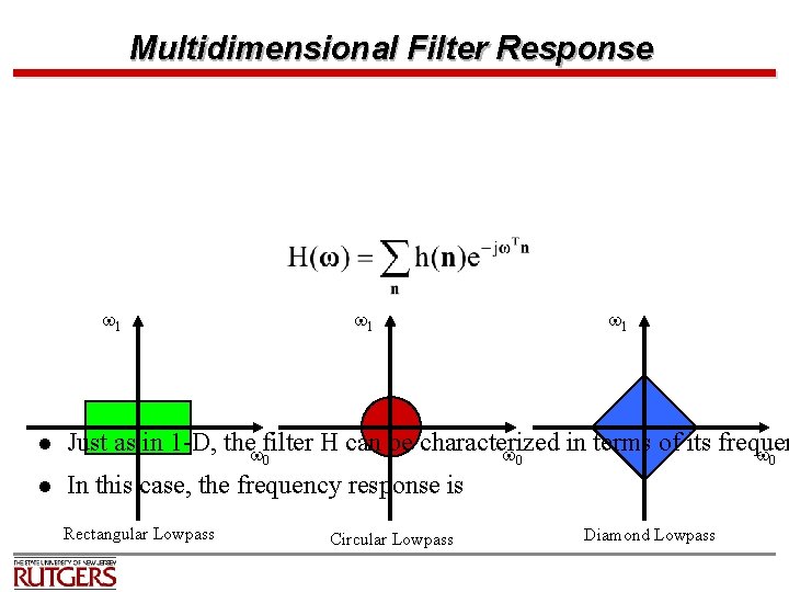
Multidimensional Filter Response w 1 w 1 l Just as in 1 -D, thewfilter H can be characterized in terms of its frequen w w l In this case, the frequency response is 0 Rectangular Lowpass 0 Circular Lowpass 0 Diamond Lowpass

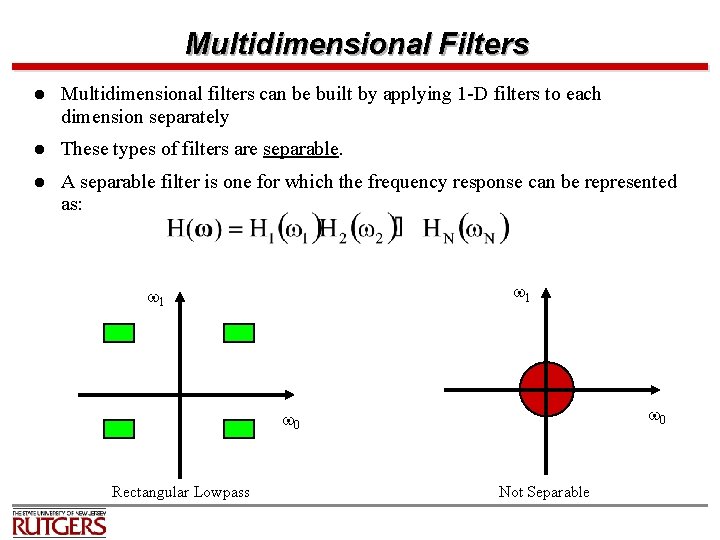
Multidimensional Filters l Multidimensional filters can be built by applying 1 -D filters to each dimension separately l These types of filters are separable. l A separable filter is one for which the frequency response can be represented as: w 1 w 0 Rectangular Lowpass Not Separable

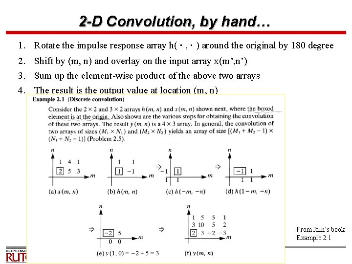
2 -D Convolution, by hand… 1. Rotate the impulse response array h( , ) around the original by 180 degree 2. Shift by (m, n) and overlay on the input array x(m’, n’) 3. Sum up the element-wise product of the above two arrays 4. The result is the output value at location (m, n) From Jain’s book Example 2. 1

For Next Time… l Next time we will focus on multidimensional sampling. – This lecture will be a blackboard/whiteboard style lecture. l To prepare, read paper provided on website, and the discussion on lattices in the textbook