Image Analogies Aaron Hertzmann 1 2 Charles E

Image Analogies Aaron Hertzmann (1, 2) Charles E. Jacobs (2) Nuria Oliver (2) Brian Curless (3) David H. Salesin (2, 3) 1 New York University 2 Microsoft Research 3 University of Washington

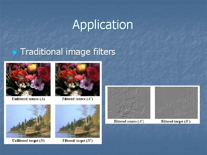
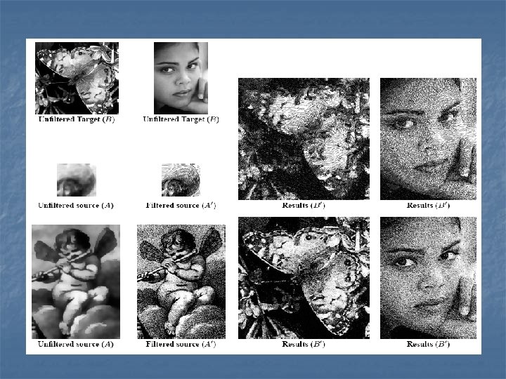
Introduction n A. nal. o. gy n n A systematic comparison between structures that uses properties of and relations between objects of a source structure to infer properties of and relations between objects of a target structure Given a pair of images A and A’ (the unfiltered and filtered source images, respectively), along with some additional unfiltered target image B, synthesize a new filtered target image B’ such that A : A’ : : B’

Introduction n We use an autoregression algorithm, based primarily on recent work in texture synthesis by Wei and Levoy and Ashikhmin. Indeed, our approach can be thought of as a combination of these two approaches, along with a generalization to the situation of corresponding pairs of images, rather than single textures. In order to allow statistics from an image A to be applied to an image B with complete different colors, we sometimes operate in a preprocessed luminance space.

Introduction n Applications: Traditional texture synthesis n Improved texture synthesis n Super-resolution n Texture transfer n Artistic filter n Texture-by-numbers n

Related work n n Machine learning for graphics Texture synthesis Non-photorealistic rendering Example-based NPR

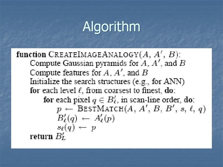
Algorithm n n n As input, our algorithm takes a set of three images, the unfiltered source image A, the filtered source image A’, and the unfiltered target image B. It produces the filtered target image B’ as output. Our approach assumes that the two source images are registered n n The colors at and around any given pixel p in A correspond to the colors at and around that same pixel p in A’ We are trying to learn the image filter

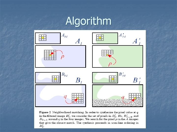
Algorithm n n n We use A(p) (or A’(p)) to denote the complete feature vector of A(p) (or A’(p)) at pixel p Similarly, We use B(q) (or B’(q)) to denote the complete feature vector of B(q) (or B’(q)) at pixel q We will need to keep track of the position p of the source pixel that was copied to pixel q of the target, we will store this addition data structure s(. ) n n For example, s(q)=p We will actually use a multiscale representation of all five of these quantities in our algorithm, we typically index each of these arrays by their multiscale level l using subscripts n For example, presents the source image A at a given resolution, then represents a corresponding lowerresolution image at the next coarser level

Algorithm n n First, in an initialization phase, multiscale (Guassian pyramid) representations of A, A’, and B is constructed, along with their feature vectors and some additional indices used for speeding the matching process. We use L to denote the maximum level (the highestresolution) At each level l, statistics pertaining to each pixel q in the target pair are compared against statistics for every pixel p in the source pair, and the “best” match is found. The pixel that matched best is recorded in

Algorithm

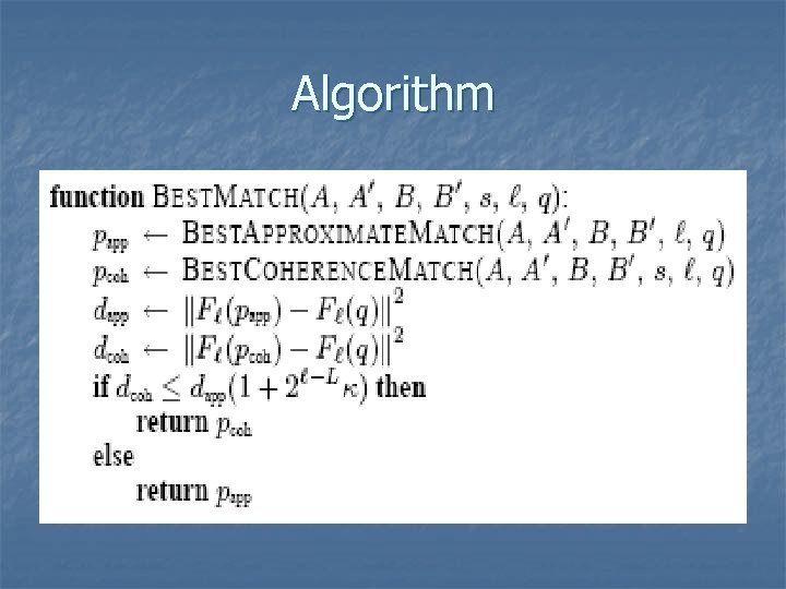
Algorithm n n The heart of the image analogies algorithm is the Best. Match subroutine The routine finds the pixel p in the source pair that best matches the pixel being synthesized, using two different approaches: n n an approximate search, which attempts to efficiently find the closest-matching pixel according to the feature vectors of p, q, and their neighborhood; a coherence search, based on Ashikhmin’s approach , which attempts to preserve coherence with the neighboring synthesized pixels

Algorithm

Algorithm n n Since L 2 -norm is imperfect measure of perceptual similarity, coherent pixels will often look better than the best match under L 2 Thus, the larger the value of , the more coherence is favored over accuracy in the synthesized image In order to keep the coherence term consistent at different scales, we attenuate it by a factor of since pixel locations at coarser scales are spaced further apart than at finer scales. We typically use for color nonphotorealistic filters, for line art filters, and for texture synthesis.

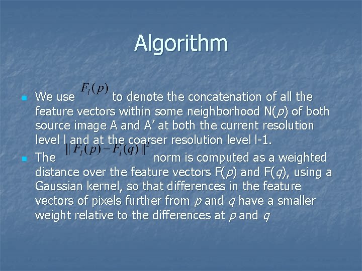
Algorithm n n We use to denote the concatenation of all the feature vectors within some neighborhood N(p) of both source image A and A’ at both the current resolution level l and at the coarser resolution level l-1. The norm is computed as a weighted distance over the feature vectors F(p) and F(q), using a Gaussian kernel, so that differences in the feature vectors of pixels further from p and q have a smaller weight relative to the differences at p and q

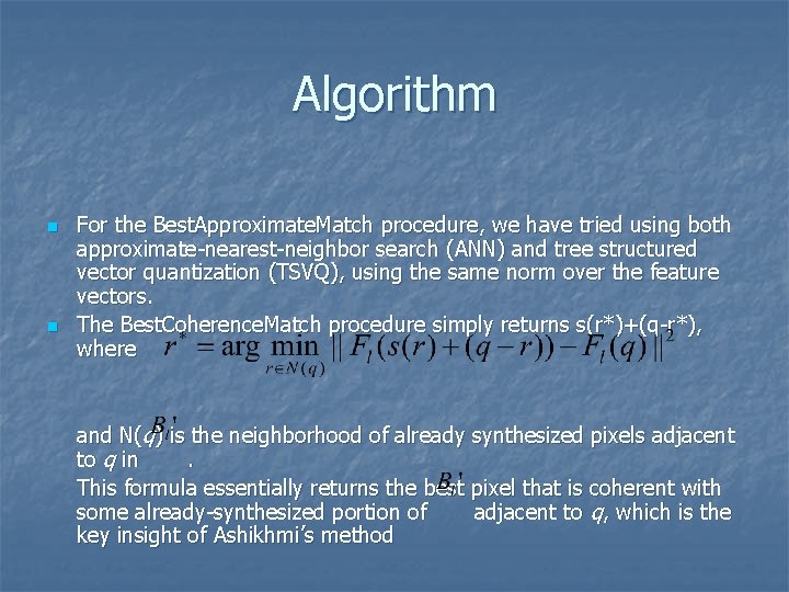
Algorithm n n For the Best. Approximate. Match procedure, we have tried using both approximate-nearest-neighbor search (ANN) and tree structured vector quantization (TSVQ), using the same norm over the feature vectors. The Best. Coherence. Match procedure simply returns s(r*)+(q-r*), where and N(q) is the neighborhood of already synthesized pixels adjacent to q in. This formula essentially returns the best pixel that is coherent with some already-synthesized portion of adjacent to q, which is the key insight of Ashikhmi’s method

Algorithm

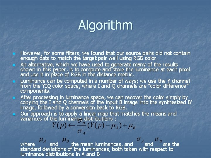
Algorithm n n n However, for some filters, we found that our source pairs did not contain enough data to match the target pair well using RGB color. An alternative, which we have used to generate many of the results shown in this paper, is to compute and store the luminance at each pixel and use it in place of RGB in the distance metric. Luminance can be computed in a number of ways; we use the Y channel from the YIQ color space, where I and Q channels are “color difference” components. After processing in luminance space, we can recover the color simply by copying the I and Q channels of the input B image into the synthesized B’ image, followed by a conversion back to RGB. Our approach is to apply a linear map that matches the means and variances of the luminance distributions : where and the mean luminances, and are the standard deviations of the luminances, both taken with respect to luminance distributions in A and B

Application n Traditional image filters

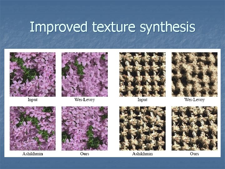
Application n Improved texture synthesis The algorithm we have described, when used in this way for texture synthesis, combines the advantages of the weighted L 2 norm and Ashikhmin’s algorithm. n For example, the synthesized textures shown in next figure have a similar high quality to those of Ashikhmin’s algorithm, without the edge discontinuities. n

Improved texture synthesis

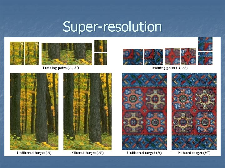
Application n Super-resolution n n Image analogies can be used to effectively “hallucinate” more detail in low-resolution images, given some low-and high-resolution pairs (used as A and A’) for small portions of the image. Training data is used to specify a “super-resolution” filter that is applied to a blurred version of the full image to recover an approximation to the higherresolution original.

Super-resolution

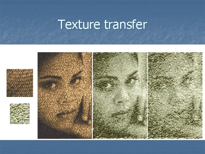
Application n Texture transfer n n n We filter an image B so that it has the texture of a given example texture A’. We can trade off the appearance between that of the unfiltered image B and that of the texture by introducing a weight into the distance metric that emphasizes similarity of the (A, B) pair over that of the (A’, B’) For better results, we also modify the neighborhood matching by usingle-scale 1*1 neighborhoods in the A and B images.

Texture transfer

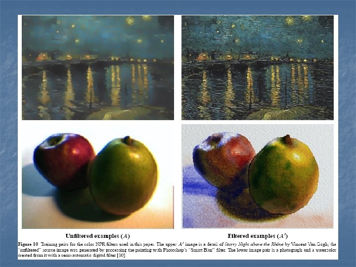
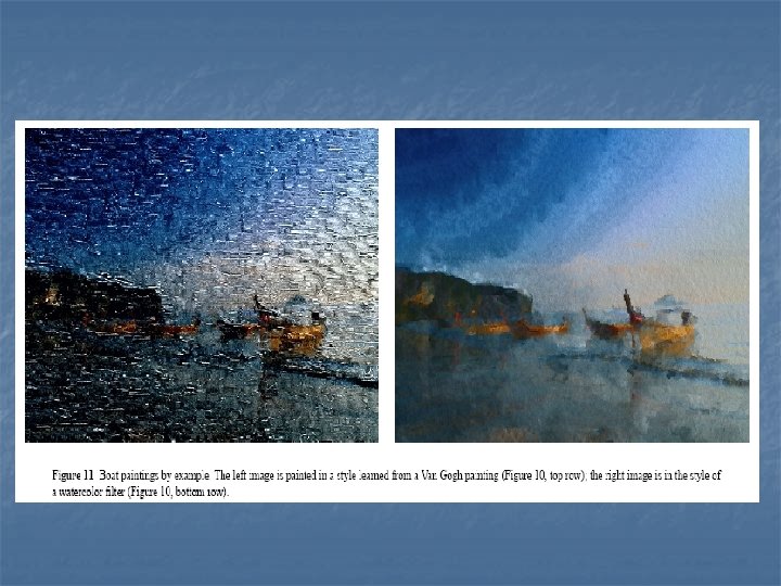
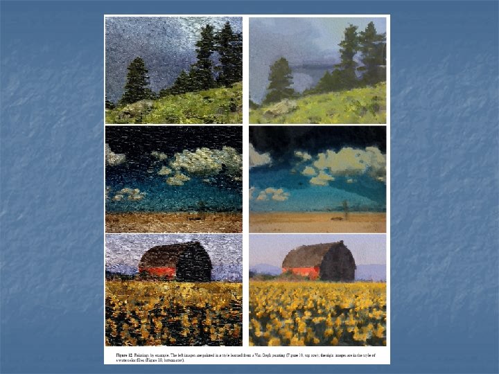
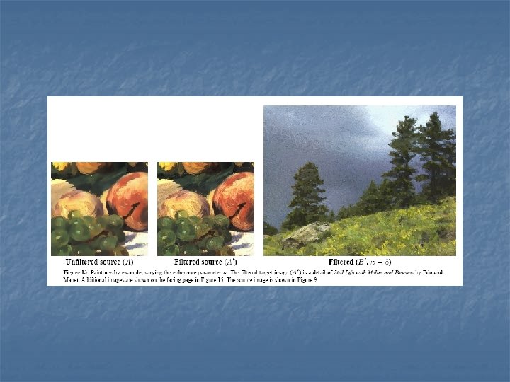
Application n Artistic filters n n n For the color artistic filters in this paper, we performed synthesis in luminance space, using the preprocessing described. For line art filters, using steerable filter responses in feature vectors leads to significant improvement. We suspect that this is because line art depends significantly on gradient directions in the input images.

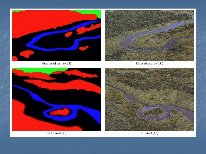
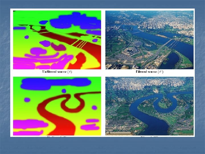
Application n Texture-by-numbers It allows new imagery to be synthesized by applying the statistics of a labeled example image to a new labeling image B. n A major advantage of texture-by-numbers is that it allows us to synthesize from images for which ordinary texture synthesis would produce poor results n

The End n http: //grail. cs. washington. edu/projects/im age-analogies