Image 2020 Fall Image Processing n Quantization Uniform

Image 2020, Fall

Image Processing n Quantization Ø Uniform Quantization Ø Halftoning & Dithering n Pixel Operation Ø Ø Add random noise Add luminance Add contrast Add saturation n Filtering Ø Blur Ø Detected edges n Warping Ø Scale Ø Rotate Ø Warp n Combining Ø Composite Ø Morph Ref] Thomas Funkhouser, Princeton Univ.

What is an Image? n An image is a 2 D rectilinear array of samples A pixel is a sample, not a little square

Image Resolution n Intensity resolution Ø Each pixel has only “Depth” bits for colors/intensities n Spatial resolution Ø Image has only “Width” x “Height” pixels n Temporal resolution Ø Monitor refreshes images at only “Rate” Hz Width x Height Depth Rate NTSC 640 x 480 8 30 Workstation 1280 x 1024 24 75 Film 3000 x 2000 12 24 Laser Printer 6600 x 5100 1 - Typical Resolutions Height Width De pt h

Source of Error n Intensity quantization Ø Not enough intensity resolution n Spatial aliasing Ø Not enough spatial resolution n Temporal aliasing Ø Not enough temporal resolution Real value Sample value

Quantization n Artifact due to limited intensity resolution Ø Frame buffers have limited number of bits per pixel Ø Physical devices have limited dynamic range

Uniform Quantization 반올림(Round)

Uniform Quantization n Image with decreasing bits per pixel

Reducing Effects of Quantization n Our eyes tend to integrate or average the fine detail into an overall intensity n Halftoning Ø A technique used in newspaper printing Ø The process of converting a continuous tone image into an image that can be printed with one color ink (grayscale) or four color inks (color) n Dithering Ø Dithering is used to create a wide variety of patterns for use as backgrounds, fills and shadings, as well as for creating halftones, and for correcting aliasing. n Halftones are created through a process called dithering Ø Dithering Methods(방법론) , Halfton result(결과물)

Classical Halftoning n Use dots of varying size to represent intensities Ø Area of dots proportional to intensity in image

Halftoning n A technique used in newspaper printing n Only two intensities are possible, blob of ink and no blob of ink n But, the size of the blob can be varied n Also, the dither patterns of small dots can be used

Classical Halftoning Original Image Halfton Image

Halfton patterns n Use cluster of pixels to represent intensity Ø Trade spatial resolution for intensity resolution 2 by 2 pixel grid patterns mask 3 by 3 pixel grid patterns

Halfton patterns

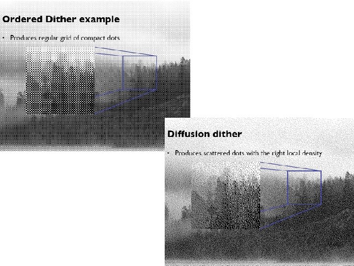
Dithering n Distribute errors among pixels Ø Exploit spatial integration in our eye Ø Display greater range of perceptible intensities

Halftoning – Moire Patterns n Ø Ø Ø Moire[more-ray] patterns Repeated use of same dot pattern for particular shade results in repeated pattern (Perceived as a moire pattern) result from overlapping repetitive elements Instead, randomize halftone pattern

Halftoning – Moire Patterns

Signal Processing (1/2) n Signal Ø Real World : Continuous Signal Ø Digital World: Discrete Signal n Image Ø spatial domain • not temporal domain • intensity variation over space

Signal Processing (2/2) n Sampling and reconstruction process Ø Sampling • The process of selecting a finite set of values from a signal • Samples (the selected values) Ø Reconstruction • recreate the original continuous signal from the samples

Sampling and Reconstruction

Aliasing n In general Ø Artifact due to under-sampling or poor reconstruction n Specifically, in graphics Ø Spatial aliasing Ø Temporal aliasing Sampling below the Nyquist rate

Nyquist rate and aliasing n Nyquist rate Ø lower bound on the sampling rate Ø Sampling at the Nyquist rate • sampling rate > 2* max frequency 주파수(frequency): 초당 사이클의 횟수(Hz)

Spatial Aliasing n Artifact due to limited spatial resolution

Spatial Aliasing n Artifact due to limited spatial resolution

Temporal Aliasing n Artifact due to limited temporal resolution Ø Spinning Backward • The wheel is spinning at 5 revolution per second – 3 rd row appear to be spinning backward at revolution per second

Temporal Aliasing n Artifact due to limited temporal resolution Ø Flickering

Anti-Aliasing n Sample at higher rate Ø Not always possible Ø Doesn’t always solve problem n Pre-filter to form bandlimited signal Ø Form bandlimited function(low-pass filter) Ø Trades aliasing for blurring

Pixel Operations n Grayscale Ø Compute luminance L Ø L=0. 30 R+0. 59 G+0. 11 B (old) • 0. 2125 R+0. 7154 G+0. 0721 B (CRT, HDTV) Original Image Grayscale Image

Pixel Operations n Negative Image Ø Simply inverse pixel components Ø Ex) RGB(5, 157, 178) RGB(250, 98, 77) Original Image Negative Image (R, G, B) (255 -R, 255 -G, 255 -B)

Pixel Operations n Adjusting Brightness Ø Simply scale pixel components • Must clamp to range (e. g. , 0 to 255) (R, G, B) (R, G , B) * scale

Pixel Operations n Adjusting Contrast Ø Compute mean luminance L for all pixels • Luminance = 0. 30* r + 0. 59*g + 0. 11*b Ø Scale deviation from L for each pixel component • Must clamp to range (e. g. , 0 to 255) R L + (R-L)*scale G L + (G-L)*scale B L + (B-L)*scale

Pixel Operations Changing Brightness Changing Contrast

Pixel Operations n Adjusting Saturation Ø Color Convert RGB HSV Ø Scale from S for each pixel component Ø Color Convert HSV RGB • Must clamp to range (e. g. , 0 to 255)

Filtering n Convolution Ø Spatial domain • Output pixel is weighted sum of pixels in neighborhood of input image • Patten of weights is the “filter”

Filtering n Convolution

Filtering n Adjust Blurriness Ø Convolve with a filter whose entries sum to one • Each pixel becomes a weighted average of its neighbors Filter Sum = 1

Filtering n Edge Detection Ø Convolve with a filter that finds differences between neighbor pixels

Filtering n Sharpening Ø Convolve with a Sharpening filter

Filtering n Embossing Ø Convert the image into grayscale Ø Convolve with a Embossing filter Ø Plus 0. 5 (128) for each pixel • Must clamp to range (e. g. , 0 to 255)

Summary n Image representation Ø A pixel is a sample, not a little square Ø Images have limited resolution n Halftoning and dithering Ø Reduce visual artifacts due to quantization Ø Distribute errors among pixels • Exploit spatial integration in our eye n Sampling and reconstruction Ø Reduce visual artifacts due to aliasing Ø Filter to avoid undersampling • Blurring is better than aliasing

Image Processing n Quantization Ø Uniform Quantization Ø Halftoning & Dithering n Pixel Operation Ø Ø Add random noise Add luminance Add contrast Add saturation n Warping Ø Scale Ø Rotate Ø Warp n Combining Ø Composite Ø Morph n Filtering Ø Blur Ø Detected edges Ref] Thomas Funkhouser, Princeton Univ.

Image Warping n Move pixels of image Ø Mapping : Specifying where every pixel goes • Forward • Reverse Ø Resampling : Computing colors at destination pixels • Point sampling • Triangle Filter • Gaussian filter

Image Warping n Two options Ø Forward mapping Ø Reverse mapping

Mapping n Define transformation Ø Describe the destination (x, y) for every location (u, v) in the source (or vice-verse, if invertible) Source (u, v) Destination (x, y)

Example Mappings n Scale by factor Ø x = factor * u Ø y = factor * v Source (u, v) Destination (x, y)

Example Mappings n Rotate by q degrees Ø x = ucosq - vsinq Ø y = usinq + vcosq Source (u, v) Destination (x, y)

Example Mappings n Shear in X by factor Ø x = u + factor * v Øy=v n Shear in Y by factor Øx=u Ø y = v + factor * u

Other Mappings n Any function of u and v Ø X = fx (u, v) Ø Y = fy (u, v)

Image Warping Implementation I n Forward mapping for (int u =0; u < umax; u++) { for (int v = 0; v < vmax; v++) { float x = fx (u, v); float y = fy (u, v); dst (x, y) = src(u, v) ; } }

Forward Mapping n Iterate over source image Ø Many source pixels can map to same destination pixel Ø Some destination pixels may not be covered

Image Warping Implementation II n Reverse mapping for (int x =0; x < xmax; x++) { for (int y = 0; y < ymax; y++) { float u = fx-1 (x, y); float v = fy-1 (x, y); dst (x, y) = src(u, v); } }

Reverse Mapping n Iterate over destination image Ø Must resample source Ø May oversample, but much simpler

Resampling n Evaluate source image at arbitrary (u, v) Ø (u, v) does not usually have integer coordinates

Resampling n Resampling Ø Point sampling Ø Triangle filter Ø Gaussain filter

Point Sampling n Take value at closest pixel Ø int iu = trunc(u + 0. 5) Ø int iv = trunc(v + 0. 5) Ø dst(x, y) = src(iu, iv) n This method is simple, but it cause aliasing

Filtering n Compute weighted sum of pixel neighborhood Ø Weights are normalized values of kernel function Ø Equivalent to convolution at samples

Triangle Filtering n Kernel is triangle function

Interpolation n Linear Interpolation (선형보간법) Ø a method of curve fitting using linear polynomials to construct new data points within the range of a discrete set of known data points. 0. 2 P 1 20 0. 8 P P 2 200 P=20*0. 8+200*0. 2

Triangle Filtering (with width = 1) n Bilinearly interpolate four closest pixels Ø a = linear interpolation of src(u 1, v 2) and src(u 2, v 2) Ø b = linear interpolation of src(u 1, v 1) and src(u 2, v 1) Ø dst = linear interpolation of “a” and “b”

Ex) Bilinear Interpolation n Bilinearly interpolate four closest pixels Øa=? Øb=? Øp=? (1, 0) 0) (1, a (1, 1) 200 100 (0. 7, 0. 2) p 50 (0, 0) 250 b (1, 0)

Gaussian Filtering n Kernel is Gaussian function Filter width =2

Filtering Methods Comparison n Trade-offs Ø Aliasing versus blurring Ø Computation speed Point Bilinear Gaussian

Image Warping Implementation n Reverse mapping for (int x =0; x < xmax; x++) { for (int y = 0; y < ymax; y++) { float u = fx-1 (x, y); float v = fy-1 (x, y); dst (x, y) = resample_src(u, v, w); } }

Example: Scale n scale (src, dst, sx, sy) : Float w = max (1. 0/sx, 1. 0/sy) for (int x =0; x < xmax; x++) { for (int y = 0; y < ymax; y++) { float u = x / sx; float v = y / sy; dst (x, y) = resample_src(u, v, w); } }

Example: Rotate n Rotate (src, dst, theta) : for (int x =0; x < xmax; x++) { for (int y = 0; y < ymax; y++) { float u = x*cos(-theta) - y*sin(-theta); float v = x*sin(-theta) + y*cos(-theta); dst (x, y) = resample_src(u, v, w); } }

Example: Fun n Swirl (src, dst, theta) : for (int x =0; x < xmax; x++) { for (int y = 0; y < ymax; y++) { float u = rot(dist(x, xcenter)*theta); float v = rot(dist(y, yecnter)*theta); dst (x, y) = resample_src(u, v, w); } }

Combining images n Image compositing Ø Blue-screen mattes Ø Alpha channel n Image morphing Ø Specifying correspondence Ø Warping Ø Blending

Image Compositing n Separate an image into “elements” Ø Render independently Ø Composite together n Application Ø Cel animation Ø Chroma-keying Ø Blue-screen matting

Blue Screen Matting n Composite foreground and background images Ø Create background image Ø Create foreground image with blue background Ø Insert non-blue foreground pixels into background n Problem : no partial coverage

Alpha Channel n Encodes pixel coverage informations Ø a = 0 no coverage (or transparent) Ø a = 1 full coverage (or opaque) Ø 0 < a < 1 partial coverage (or semi-transparent) n Example: a = 0. 3

Composite with Alpha n Composite with Alpha Ø Control the linear interpolation of foreground and background pixels when elements are composited

Alpha Blending: “Over” Operator n Alpha channel convention Ø (r, g, b, a) represents a pixel that is a covered by A the color C = (r*a, g*a, b*a) • Color components are premultiplied by a • Can display (r, g, b) value directly • Closure in composition algebra A = (r. A , g. A, b. A) a. AA = (r. A*a. A , g. A*a. A, b. A*a. A) B

Semi-Transparent Objects n Suppose we put A over B over background G Ø How much of B is blocked by A ? a. A Ø How much of B show through A ? (1 -a. A) Ø How much of G shows through both A and B ? (1 -a. A) (1 -a. B) Ø αAA+ (1 -αA)αBB+ (1 -αA)(1 -αB)G = αAA + (1 - αA) [αBB + (1 -αB)G] = A over[B over G]

Image Morphing n Animate transition between two images

Cross-Dissolving n Blend images with “over” operator Ø alpha of bottom image is 1. 0 Ø alpha of top image varies from 0. 0 to 1. 0 blend(i, j) = (1 -t) src(i, j) + t dst(i, j) (0 <= t <= 1)

Image Morphing n Combines warping and cross-disolving

Feature Based Morphing n Beier & Neeley use pairs of lines to specify warp Ø Given p in dst image, where is p’ in source image ?

Feature Based Morphing Feature Matching Image Warping Morphed Image

Feature Based Morphing Warping Morphing Black Or White-Michael Jackson

Image Processing n Quantization Ø Uniform Quantization Ø Halftoning & Dithering n Pixel Operation Ø Ø Add random noise Add luminance Add contrast Add saturation n Filtering Ø Blur Ø Detected edges n Warping Ø Scale Ø Rotate Ø Warp n Combining Ø Composite Ø Morph Ref] Thomas Funkhouser, Princeton Univ.