II Deviations from HWE A Mutation B Migration

II. Deviations from HWE A. Mutation B. Migration C. Non-Random Mating D. Genetic Drift - Sampling Error E. Selection 1. Measuring “fitness” – differential reproductive success

II. Deviations from HWE A. Mutation B. Migration C. Non-Random Mating D. Genetic Drift - Sampling Error E. Selection 1. Measuring “fitness” – differential reproductive success a. The mean number of reproducing offspring (or females)/female

II. Deviations from HWE A. Mutation B. Migration C. Non-Random Mating D. Genetic Drift - Sampling Error E. Selection 1. Measuring “fitness” – differential reproductive success a. The mean number of reproducing offspring (or females)/female b. Components of fitness:

II. Deviations from HWE A. Mutation B. Migration C. Non-Random Mating D. Genetic Drift - Sampling Error E. Selection 1. Measuring “fitness” – differential reproductive success a. The mean number of reproducing offspring (or females)/female b. Components of fitness - probability of female surviving to reproductive age

II. Deviations from HWE A. Mutation B. Migration C. Non-Random Mating D. Genetic Drift - Sampling Error E. Selection 1. Measuring “fitness” – differential reproductive success a. The mean number of reproducing offspring (or females)/female b. Components of fitness - probability of female surviving to reproductive age - number of offspring the female produces

II. Deviations from HWE A. Mutation B. Migration C. Non-Random Mating D. Genetic Drift - Sampling Error E. Selection 1. Measuring “fitness” – differential reproductive success a. The mean number of reproducing offspring (or females)/female b. Components of fitness - probability of female surviving to reproductive age - number of offspring the female produces - probability that offspring survive to reproductive age

II. Deviations from HWE A. Mutation B. Migration C. Non-Random Mating D. Genetic Drift - Sampling Error E. Selection 1. Measuring “fitness” – differential reproductive success a. The mean number of reproducing offspring (or females)/female b. Components of fitness - probability of female surviving to reproductive age - number of offspring the female produces - probability that offspring survive to reproductive age c. With a limited energy budget, selection cannot maximize all three components… there will necessarily be TRADE-OFFS.

E. Selection 1. Measuring “fitness” – differential reproductive success 2. Relationships with Energy Budgets

E. Selection 1. Measuring “fitness” – differential reproductive success 2. Relationships with Energy Budgets GROWTH METABOLISM REPRODUCTION

E. Selection 1. Measuring “fitness” – differential reproductive success 2. Relationships with Energy Budgets Maximize probability of survival Maximize reproduction GROWTH METABOLISM REPRODUCTION

E. Selection 1. Measuring “fitness” – differential reproductive success 2. Relationships with Energy Budgets Trade-offs within reproduction REPRODUCTION METABOLISM Lots of small, low prob of survival A few large, high prob of survival

E. Selection 1. Measuring “fitness” – differential reproductive success 2. Relationships with Energy Budgets 3. Modeling Selection

3. Modeling Selection for a Dominant Allele p = 0. 4, q = 0. 6 AA Aa aa Parental "zygotes" 0. 16 0. 48 0. 36 = 1. 00

3. Modeling Selection for a Dominant Allele p = 0. 4, q = 0. 6 AA Aa aa Parental "zygotes" 0. 16 0. 48 0. 36 prob. of survival (fitness) 0. 8 0. 2 = 1. 00

3. Modeling Selection for a Dominant Allele p = 0. 4, q = 0. 6 AA Aa aa Parental "zygotes" 0. 16 0. 48 0. 36 prob. of survival (fitness) 0. 8 0. 2 Relative Fitness 1 1 0. 25 = 1. 00

3. Modeling Selection for a Dominant Allele p = 0. 4, q = 0. 6 AA Aa aa Parental "zygotes" 0. 16 0. 48 0. 36 prob. of survival (fitness) 0. 8 0. 2 Relative Fitness 1 1 0. 25 Survival to Reproduction 0. 16 0. 48 0. 09 = 1. 00

3. Modeling Selection for a Dominant Allele p = 0. 4, q = 0. 6 AA Aa aa Parental "zygotes" 0. 16 0. 48 0. 36 prob. of survival (fitness) 0. 8 0. 2 Relative Fitness 1 1 0. 25 Survival to Reproduction 0. 16 0. 48 0. 09 = 1. 00 = 0. 73

3. Modeling Selection for a Dominant Allele p = 0. 4, q = 0. 6 AA Aa aa Parental "zygotes" 0. 16 0. 48 0. 36 prob. of survival (fitness) 0. 8 0. 2 Relative Fitness 1 1 0. 25 Survival to Reproduction 0. 16 0. 48 0. 09 = 0. 73 Geno. Freq. , breeders 0. 22 0. 66 0. 12 = 1. 00

3. Modeling Selection for a Dominant Allele p = 0. 4, q = 0. 6 AA Aa aa Parental "zygotes" 0. 16 0. 48 0. 36 prob. of survival (fitness) 0. 8 0. 2 Relative Fitness 1 1 0. 25 Survival to Reproduction 0. 16 0. 48 0. 09 = 0. 73 Geno. Freq. , breeders 0. 22 0. 66 0. 12 = 1. 00 Gene Freq's, gene pool p = 0. 55 q = 0. 45 = 1. 00

3. Modeling Selection for a Dominant Allele p = 0. 4, q = 0. 6 AA Aa aa Parental "zygotes" 0. 16 0. 48 0. 36 prob. of survival (fitness) 0. 8 0. 2 Relative Fitness 1 1 0. 25 Survival to Reproduction 0. 16 0. 48 0. 09 = 0. 73 Geno. Freq. , breeders 0. 22 0. 66 0. 12 = 1. 00 Gene Freq's, gene pool p = 0. 55 Genotypes, F 1 0. 3025 = 1. 00 q = 0. 45 0. 495 0. 2025 = 100

3. Modeling Selection for a Dominant Allele Δp declines with each generation.

3. Modeling Selection for a Dominant Allele Δp declines with each generation. BECAUSE: as q declines, a greater proportion of q alleles are present in heterozygotes (and invisible to selection). As q declines, q 2 declines more rapidly. . .

3. Modeling Selection for a Dominant Allele Δp declines with each generation. So, in large populations, it is hard for selection to completely eliminate a deleterious allele. .

3. Modeling Selection for a Dominant Allele Δp declines with each generation. Rate of change depends on the strength of selection; the difference in reproductive success among genotypes. In this case, a new adaptive mutant allele has been produced in the population. The “selection differential”, s, is selection AGAINST the existing allele that had become ‘fixed’ in the population (f = 1. 0) So, the “better” the new allele is (represented by the greater selective differential against the old allele), the faster the new mutant accumulates in the population.

3. Modeling Selection for a Dominant Allele Selection for an allele where there is not complete dominance: - Consider incomplete dominance, codominance, or heterosis. In these situations, the heterozygote has a phenotype that differs from either of the homozygotes, and selection can favor one genotype over another: - Selection might favor one homozygote over the heterozygote and other homozygote (first example), or might favor the heterozygote over the homozygotes (second example), or might favor both homozygotes over the heterozygote (not considered here).

Selection for the homozygote of a non-dominant allele p = 0. 4, q = 0. 6 AA Aa aa Parental "zygotes" 0. 16 0. 48 0. 36 prob. of survival (fitness) 0. 8 0. 4 0. 2 Relative Fitness 1 0. 5 0. 25 Survival to Reproduction 0. 16 0. 24 0. 09 = 0. 49 Geno. Freq. , breeders 0. 33 0. . 50 0. 17 = 1. 00 Gene Freq's, gene pool p = 0. 58 Genotypes, F 1 0. 34 = 1. 00 q = 0. 42 0. 48 0. 18 = 100

Selection for the homozygote of a non-dominant allele - deleterious alleles can no longer hide in the heterozygote; its presence always causes a reduction in fitness, and so it can be eliminated from a population.

Selection for the heterozygote p = 0. 4, q = 0. 6 AA Aa aa Parental "zygotes" 0. 16 0. 48 0. 36 prob. of survival (fitness) 0. 4 0. 8 0. 2 Relative Fitness 0. 5 (1 -s) 1 0. 25 (1 -t) Survival to Reproduction 0. 08 0. 48 0. 09 = 0. 65 Geno. Freq. , breeders 0. 12 0. 74 0. 14 = 1. 00 Gene Freq's, gene pool p = 0. 49 Genotypes, F 1 0. 24 q = 0. 51 0. 50 0. 26 Maintains both genes in the gene pool peq = t/s+t = 0. 75/1. 25 = 0. 6 AA = 1. 00 Aa aa = 100

Maintains both genes in the gene pool peq = t/s+t = 0. 75/1. 25 = 0. 6

Selection for the Heterozygote Sickle cell caused by a SNP of valine for glutamic acid at the 6 th position in the beta globin protein in hemoglobin (147 amino acids long). NN NS SS The malarial parasite (Plasmodium falciparum) cannot complete development in red blood cells with this hemoglobin, because O 2 levels are too low in these cells.

E. Selection 1. Measuring “fitness” – differential reproductive success 2. Relationships with Energy Budgets 3. Modeling Selection 4. Types of Selection - Selection acts on phenotypes, which may be single gene traits, polygenic quantitative traits, and/or effected by epistatic interactions. - The different effects are measured by changes in the mean phenotype over time.

E. Selection 4. Types of Selection - Directional

E. Selection 4. Types of Selection - Directional

E. Selection 4. Types of Selection - Stabilizing

E. Selection 4. Types of Selection - Disruptive Lab experiment – “bidirectional selection” – create two lines by directionally selecting for extremes. Populations are ‘isolated’ and don’t reproduce.

E. Selection 4. Types of Selection - Disruptive African Fire-Bellied Seed Crackers

Evolutionary Genetics

Evolutionary Genetics I. Speciation A. Definition: Mayr’s ‘biological species concept’ – “a group of actually or potentially interbreeding organisms that is reproductively isolated from other such groups”.

Evolutionary Genetics I. Speciation A. Definition: Mayr’s ‘biological species concept’ – “a group of actually or potentially interbreeding organisms that is reproductively isolated from other such groups”. - only appropriate for sexually reproducing species - Reproductive isolation will inevitably lead to greater genetic divergence (even just by chance), and an increased likelihood of genetic uniqueness/incompatibility.

Evolutionary Genetics I. Speciation II. Making Species - Reproductive Isolation A. Pre-Zygotic Barriers 1. Geographic Isolation (large scale or habitat)

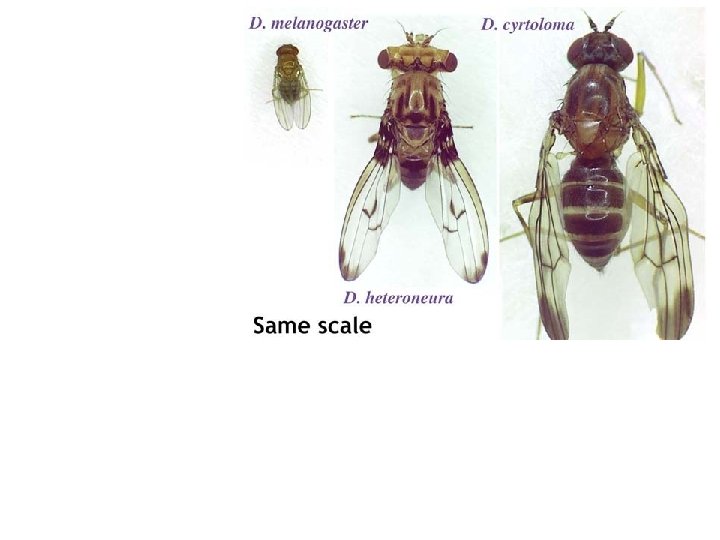
Drosophila speciation on the Hawaiian Islands. Recent divergences involve a specie colonizing a new island (Hawai’i); older divergence occurred in the past, when older islands first crested above the ocean and Obbard D J et al. Mol Biol Evol 2012; 29: 3459 -3473 were made available for colonization. © The Author 2012. Published by Oxford University Press on behalf of the Society for Molecular Biology and Evolution.

Vicariance – the splitting of a range by a new geographic feature, such as a river or land mass (next).

Almost all most recent divergence events date to 3 my, and separate species on either side of the isthmus; suggesting that the formation of the isthmus was a cause of speciation in all these species pairs. Snapping ‘Pistol’ Shrimp

Mayr – Peripatric Speciation Small population in new environment; the effect of drift and selection will cause rapid change, resulting in a speciation event.

Evolutionary Genetics II. Making Species - Reproductive Isolation A. Pre-Zygotic Barriers 1. Geographic Isolation (large scale or habitat) 2. Temporal Isolation

Evolutionary Genetics II. Making Species - Reproductive Isolation A. Pre-Zygotic Barriers 1. Geographic Isolation (large scale or habitat) 2. Temporal Isolation 3. Behavior Isolation - don't recognize one another as mates Western Meadowlark Eastern Meadowlark

Evolutionary Genetics II. Making Species - Reproductive Isolation A. Pre-Zygotic Barriers 1. Geographic Isolation (large scale or habitat) 2. Temporal Isolation 3. Behavior Isolation - don't recognize one another as mates 4. Mechanical isolation - genitalia don't fit; limit pollinators You’re cute… You’re crazy…

Evolutionary Genetics II. Making Species - Reproductive Isolation A. Pre-Zygotic Barriers 1. Geographic Isolation (large scale or habitat) 2. Temporal Isolation 3. Behavior Isolation - don't recognize one another as mates 4. Mechanical isolation - genitalia don't fit; limit pollinators 5. Gametic Isolation - gametes transferred but sperm can't fertilize egg; this is a common isolation mechanism in species that spawn at the same time