IFT 6255 Information Retrieval Text classification 1 Overview

IFT 6255: Information Retrieval Text classification 1

Overview • • Definition of text classification Important processes in classification Classification algorithms Advantages and disadvantages of algorithms • Performance comparison of algorithms • Conclusion 2

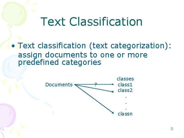
Text Classification • Text classification (text categorization): assign documents to one or more predefined categories Documents ? classes class 1 class 2. . . classn 3

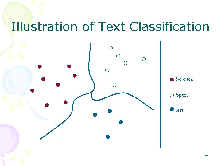
Illustration of Text Classification Science Sport Art 4

Applications of Text Classification • • • Organize web pages into hierarchies Domain specific information extraction Sort email into different folders Find interests of users Etc. 5

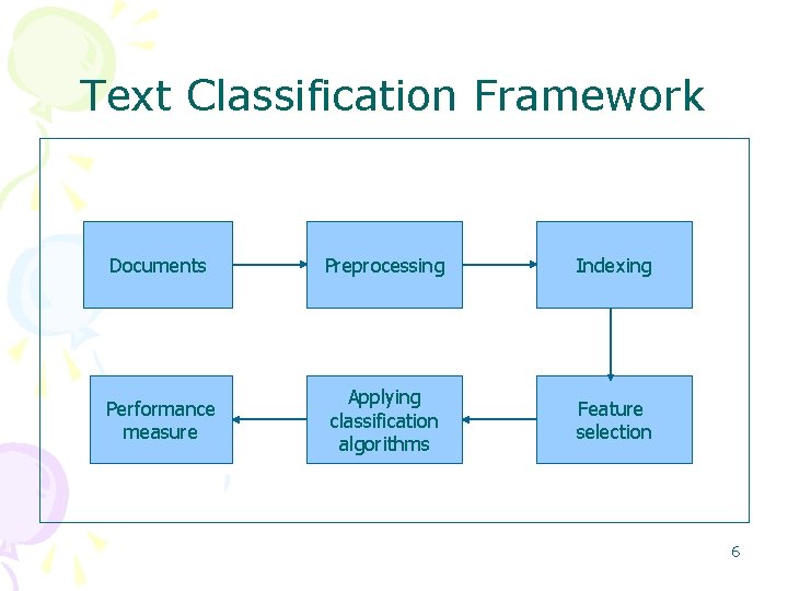
Text Classification Framework Documents Preprocessing Indexing Performance measure Applying classification algorithms Feature selection 6

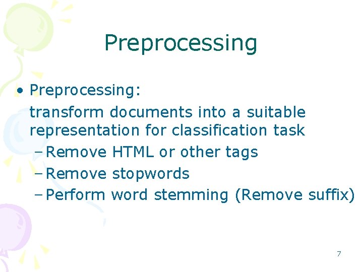
Preprocessing • Preprocessing: transform documents into a suitable representation for classification task – Remove HTML or other tags – Remove stopwords – Perform word stemming (Remove suffix) 7

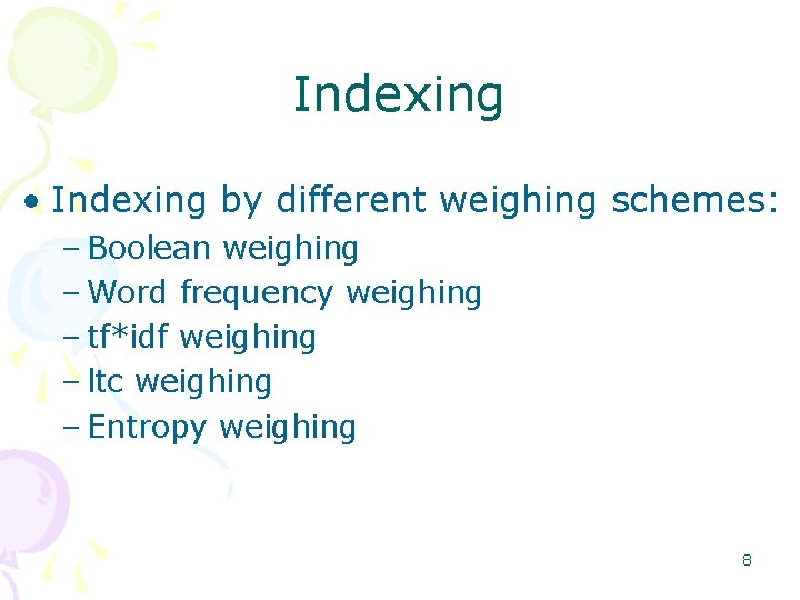
Indexing • Indexing by different weighing schemes: – Boolean weighing – Word frequency weighing – tf*idf weighing – ltc weighing – Entropy weighing 8

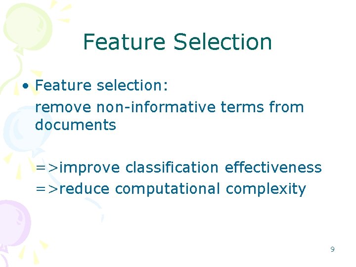
Feature Selection • Feature selection: remove non informative terms from documents =>improve classification effectiveness =>reduce computational complexity 9

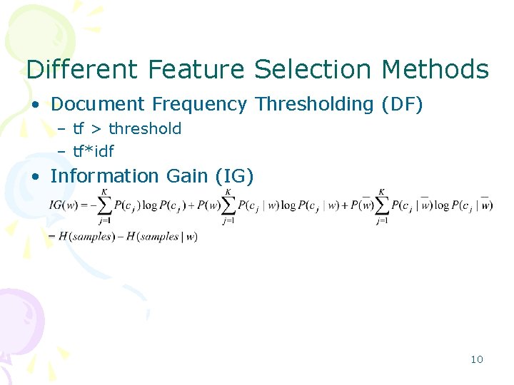
Different Feature Selection Methods • Document Frequency Thresholding (DF) – tf > threshold – tf*idf • Information Gain (IG) 10

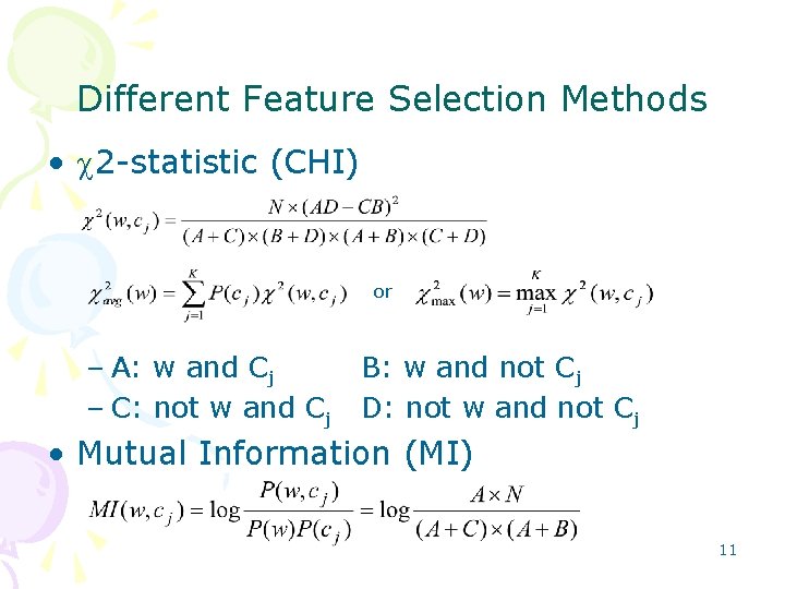
Different Feature Selection Methods • 2 statistic (CHI) or – A: w and Cj – C: not w and Cj B: w and not Cj D: not w and not Cj • Mutual Information (MI) 11

Classification Algorithms • • Rocchio’s algorithm K Nearest Neighbor algorithm (KNN) Decision Tree algorithm (DT) Naive Bayes algorithm (NB) Artificial Neural Network (ANN) Support Vector Machine (SVM) Voting algorithms 12

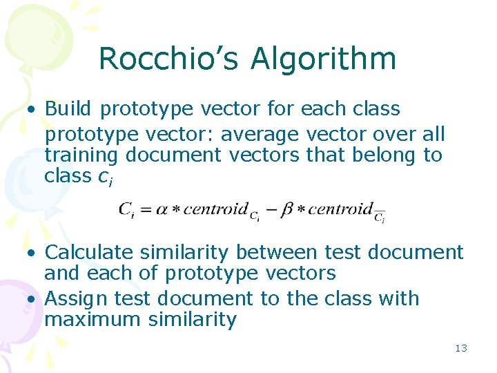
Rocchio’s Algorithm • Build prototype vector for each class prototype vector: average vector over all training document vectors that belong to class ci • Calculate similarity between test document and each of prototype vectors • Assign test document to the class with maximum similarity 13

Analysis of Rocchio’s Algorithm • Advantages: – Easy to implement – Very fast learner – Relevance feedback mechanism • Disadvantages: – Low classification accuracy – Linear combination too simple for classification – Constant and are empirical 14

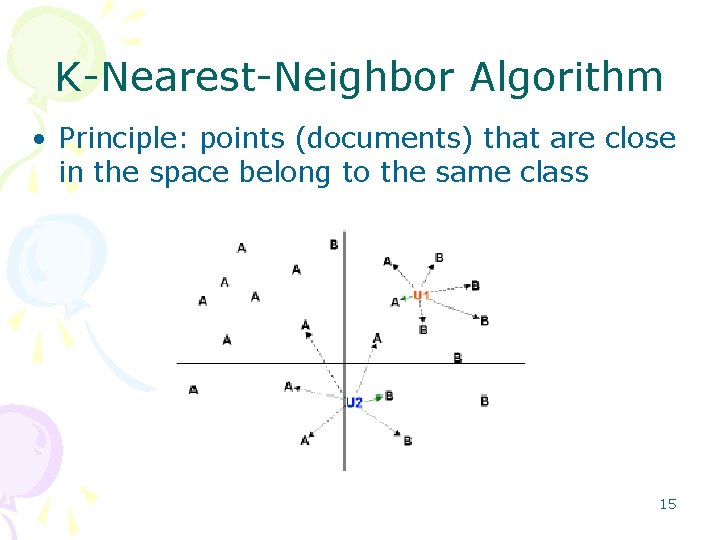
K Nearest Neighbor Algorithm • Principle: points (documents) that are close in the space belong to the same class 15

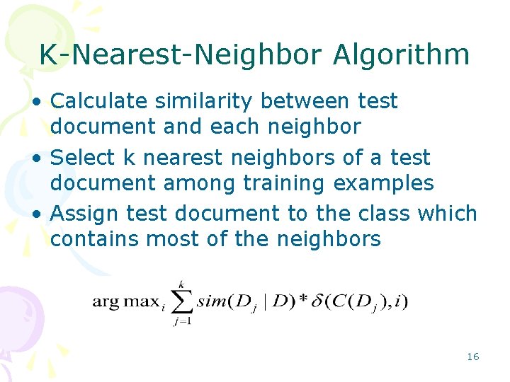
K Nearest Neighbor Algorithm • Calculate similarity between test document and each neighbor • Select k nearest neighbors of a test document among training examples • Assign test document to the class which contains most of the neighbors 16

Analysis of KNN Algorithm • Advantages: – Effective – Non parametric – More local characteristics of document are considered comparing with Rocchio • Disadvantages: – Classification time is long – Difficult to find optimal value of k 17

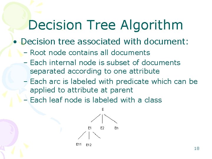
Decision Tree Algorithm • Decision tree associated with document: – Root node contains all documents – Each internal node is subset of documents separated according to one attribute – Each arc is labeled with predicate which can be applied to attribute at parent – Each leaf node is labeled with a class 18

Decision Tree Algorithm • Recursive partition procedure from root node • Set of documents separated into subsets according to an attribute • Use the most discriminative attribute first (highest IG) • Pruning to deal with overfitting 19

Analysis of Decision Tree Algorithm • Advantages: – Easy to understand – Easy to generate rules – Reduce problem complexity • Disadvantages: – Training time is relatively expensive – A document is only connected with one branch – Once a mistake is made at a higher level, any subtree is wrong – Does not handle continuous variable well – May suffer from overfitting 20

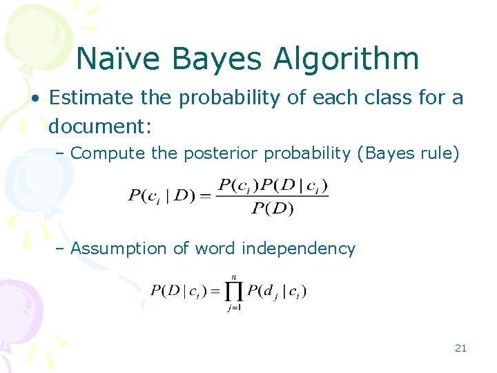
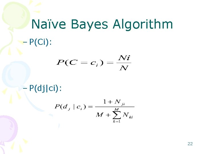
Naïve Bayes Algorithm • Estimate the probability of each class for a document: – Compute the posterior probability (Bayes rule) – Assumption of word independency 21

Naïve Bayes Algorithm – P(Ci): – P(dj|ci): 22

Analysis of Naïve Bayes Algorithm • Advantages: – Work well on numeric and textual data – Easy to implement and computation comparing with other algorithms • Disadvantages: – Conditional independence assumption is violated by real world data, perform very poorly when features are highly correlated 23

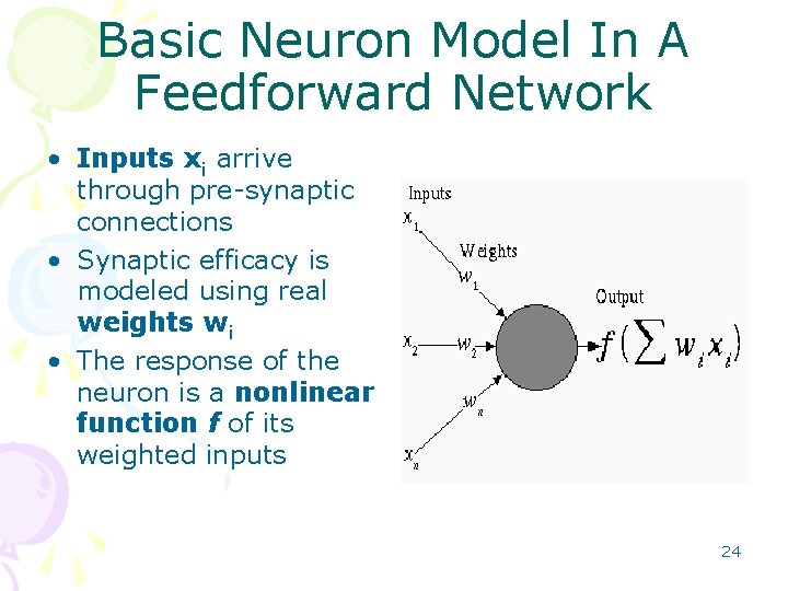
Basic Neuron Model In A Feedforward Network • Inputs xi arrive through pre synaptic connections • Synaptic efficacy is modeled using real weights wi • The response of the neuron is a nonlinear function f of its weighted inputs 24

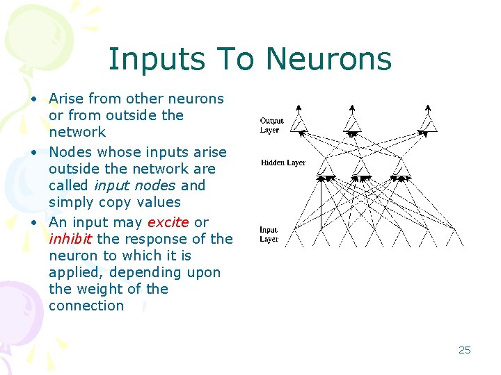
Inputs To Neurons • Arise from other neurons or from outside the network • Nodes whose inputs arise outside the network are called input nodes and simply copy values • An input may excite or inhibit the response of the neuron to which it is applied, depending upon the weight of the connection 25

Weights • Represent synaptic efficacy and may be excitatory or inhibitory • Normally, positive weights are considered as excitatory while negative weights are thought of as inhibitory • Learning is the process of modifying the weights in order to produce a network that performs some function 26

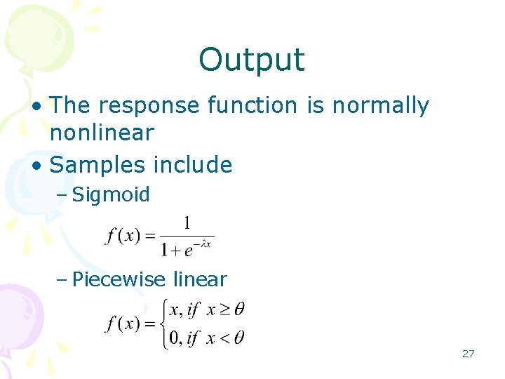
Output • The response function is normally nonlinear • Samples include – Sigmoid – Piecewise linear 27

Backpropagation Preparation • Training Set A collection of input output patterns that are used to train the network • Testing Set A collection of input output patterns that are used to assess network performance • Learning Rate-η A scalar parameter, analogous to step size in numerical integration, used to set the rate of adjustments 28

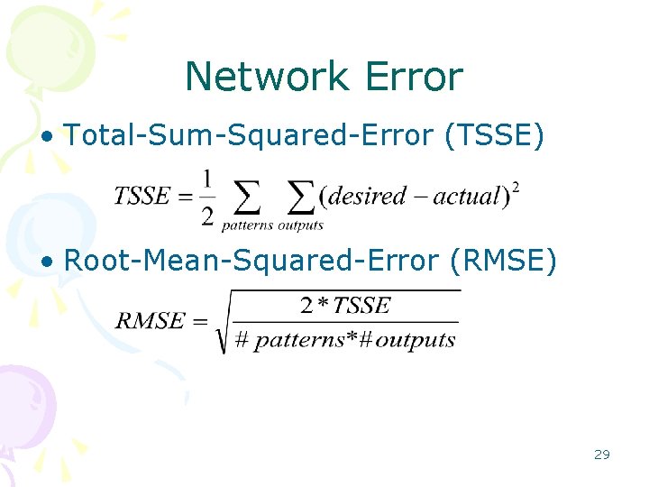
Network Error • Total Sum Squared Error (TSSE) • Root Mean Squared Error (RMSE) 29

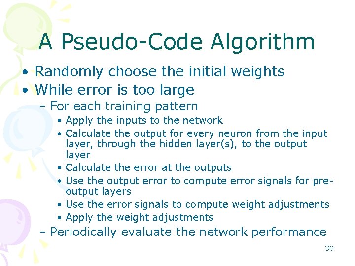
A Pseudo Code Algorithm • Randomly choose the initial weights • While error is too large – For each training pattern • Apply the inputs to the network • Calculate the output for every neuron from the input layer, through the hidden layer(s), to the output layer • Calculate the error at the outputs • Use the output error to compute error signals for pre output layers • Use the error signals to compute weight adjustments • Apply the weight adjustments – Periodically evaluate the network performance 30

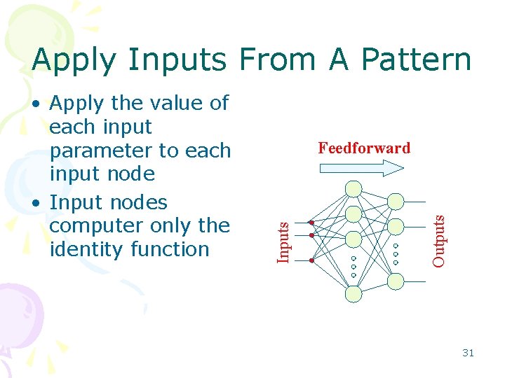
Apply Inputs From A Pattern Outputs Feedforward Inputs • Apply the value of each input parameter to each input node • Input nodes computer only the identity function 31

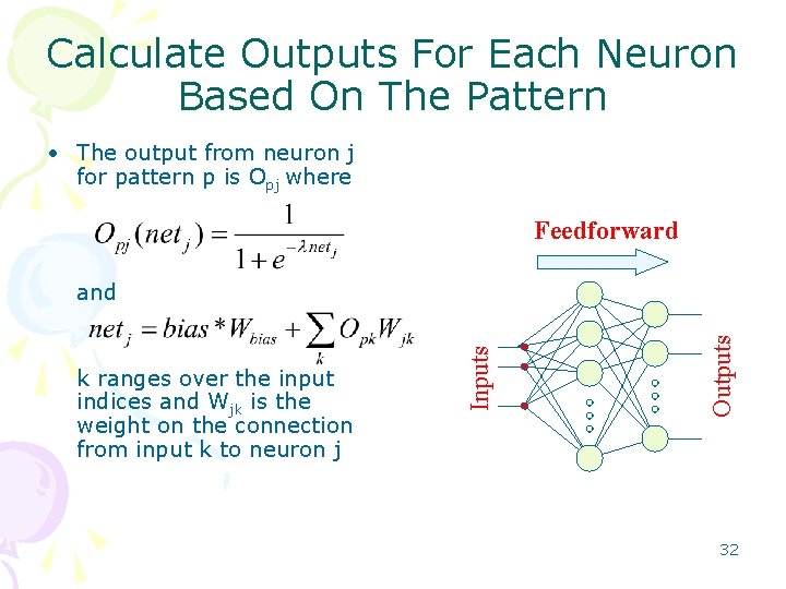
Calculate Outputs For Each Neuron Based On The Pattern • The output from neuron j for pattern p is Opj where Feedforward Outputs k ranges over the input indices and Wjk is the weight on the connection from input k to neuron j Inputs and 32

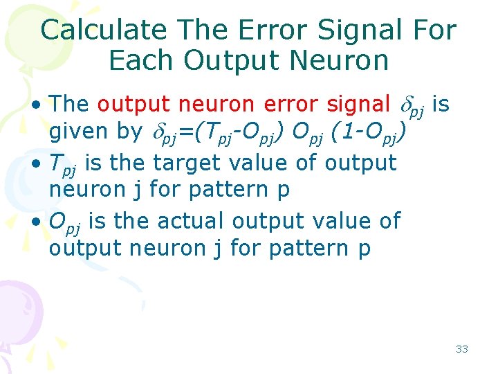
Calculate The Error Signal For Each Output Neuron • The output neuron error signal dpj is given by dpj=(Tpj-Opj) Opj (1 -Opj) • Tpj is the target value of output neuron j for pattern p • Opj is the actual output value of output neuron j for pattern p 33

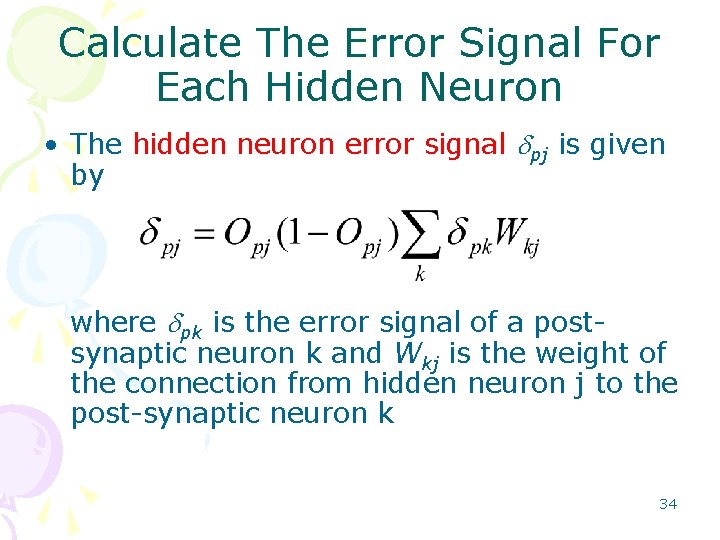
Calculate The Error Signal For Each Hidden Neuron • The hidden neuron error signal dpj is given by where dpk is the error signal of a post synaptic neuron k and Wkj is the weight of the connection from hidden neuron j to the post synaptic neuron k 34

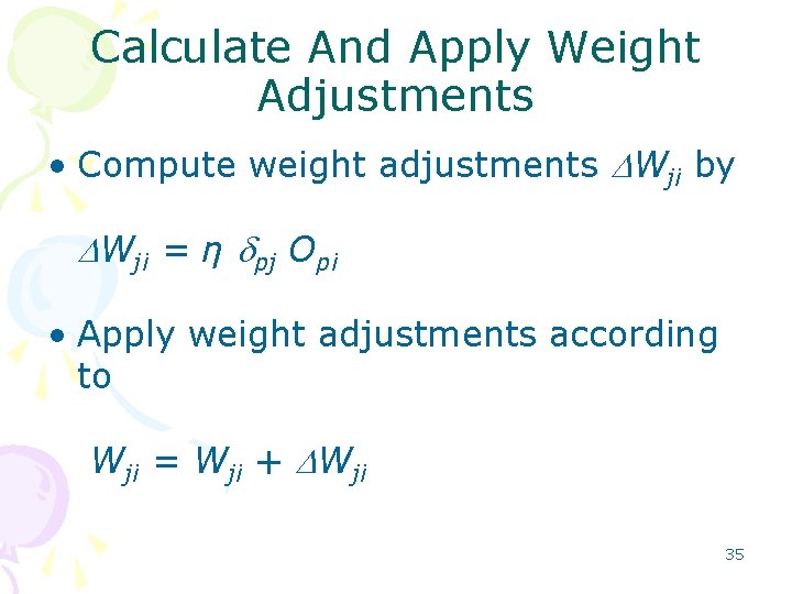
Calculate And Apply Weight Adjustments • Compute weight adjustments DWji by DWji = η dpj Opi • Apply weight adjustments according to Wji = Wji + DWji 35

Analysis of ANN Algorithm • Advantages: – Produce good results in complex domains – Suitable for both discrete and continuous data (especially better for the continuous domain) – Testing is very fast • Disadvantages: – Training is relatively slow – Learned results are difficult for users to interpret than learned rules (comparing with DT) – Empirical Risk Minimization (ERM) makes ANN try to minimize training error, may lead to overfitting 36

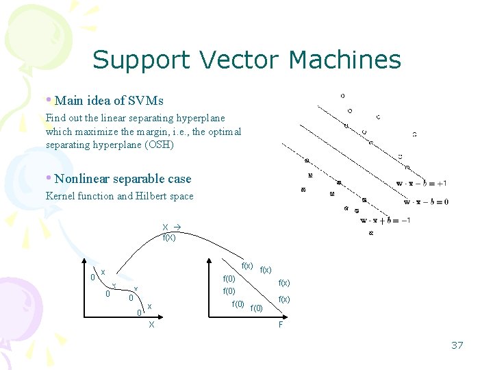
Support Vector Machines • Main idea of SVMs Find out the linear separating hyperplane which maximize the margin, i. e. , the optimal separating hyperplane (OSH) • Nonlinear separable case Kernel function and Hilbert space X f(X) 0 f(x) x 0 f(0) x 0 f(x) f(0) x X f(0) f(x) F 37

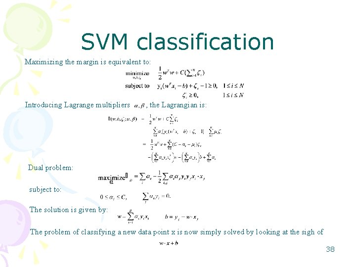
SVM classification Maximizing the margin is equivalent to: Introducing Lagrange multipliers , the Lagrangian is: Dual problem: subject to: The solution is given by: The problem of classifying a new data point x is now simply solved by looking at the sigh of 38

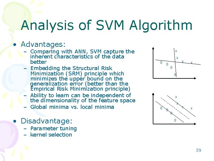
Analysis of SVM Algorithm • Advantages: – Comparing with ANN, SVM capture the inherent characteristics of the data better – Embedding the Structural Risk Minimization (SRM) principle which minimizes the upper bound on the generalization error (better than the Empirical Risk Minimization principle) – Ability to learn can be independent of the dimensionality of the feature space – Global minima vs. local minima • Disadvantage: x x 0 0 – Parameter tuning – kernel selection 39

Voting Algorithm Principle: using multiple evidence (multiple poor classifiers=> single good classifier) • Generate some base classifiers • Combine them to make the final decision 40

Bagging Algorithm • Use multiple versions of a training set D of size N, each created by resampling N examples from D with bootstrap • Each of data sets is used to train a base classifier, the final classification decision is made by the majority voting of these classifiers 41

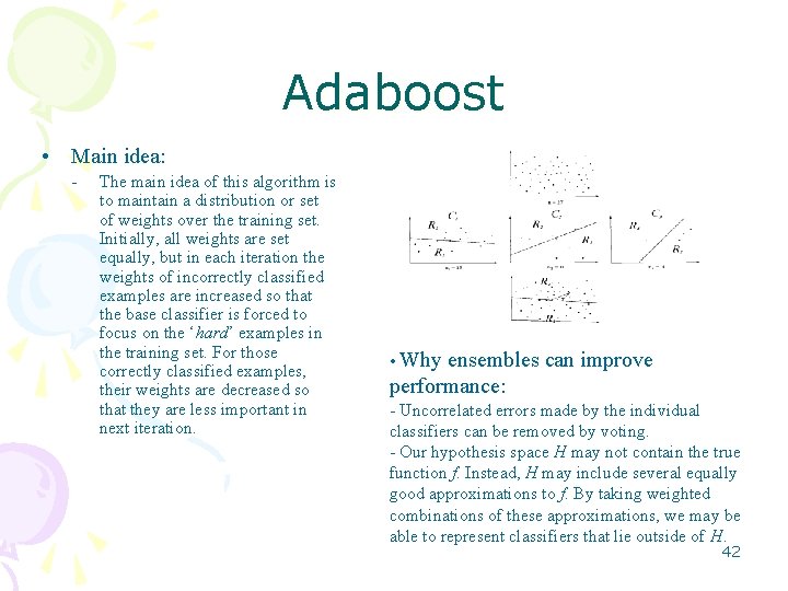
Adaboost • Main idea: - The main idea of this algorithm is to maintain a distribution or set of weights over the training set. Initially, all weights are set equally, but in each iteration the weights of incorrectly classified examples are increased so that the base classifier is forced to focus on the ‘hard’ examples in the training set. For those correctly classified examples, their weights are decreased so that they are less important in next iteration. • Why ensembles can improve performance: - Uncorrelated errors made by the individual classifiers can be removed by voting. - Our hypothesis space H may not contain the true function f. Instead, H may include several equally good approximations to f. By taking weighted combinations of these approximations, we may be able to represent classifiers that lie outside of H. 42

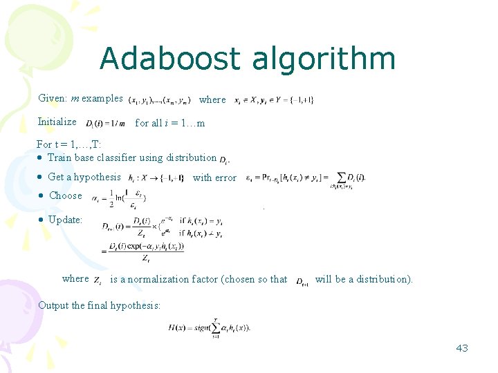
Adaboost algorithm Given: m examples Initialize where for all i = 1…m For t = 1, …, T: Train base classifier using distribution Get a hypothesis with error Choose. Update: where is a normalization factor (chosen so that will be a distribution). Output the final hypothesis: 43

Analysis of Voting Algorithms • Advantage: – Surprisingly effective – Robust to noise – Decrease the overfitting effect • Disadvantage: – Require more calculation and memory 44

Performance Measure • Performance of algorithm: – Training time – Testing time – Classification accuracy • Precision, Recall • Micro average / Macro average • Breakeven: precision = recall Goal: high classification quality and computation efficiency 45

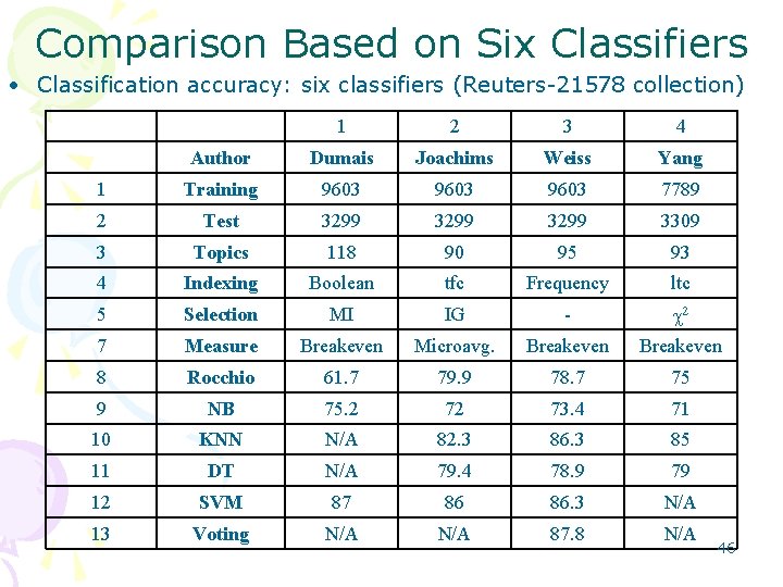
Comparison Based on Six Classifiers • Classification accuracy: six classifiers (Reuters 21578 collection) 1 2 3 4 Author Dumais Joachims Weiss Yang 1 Training 9603 7789 2 Test 3299 3309 3 Topics 118 90 95 93 4 Indexing Boolean tfc Frequency ltc 5 Selection MI IG - 2 7 Measure Breakeven Microavg. Breakeven 8 Rocchio 61. 7 79. 9 78. 7 75 9 NB 75. 2 72 73. 4 71 10 KNN N/A 82. 3 86. 3 85 11 DT N/A 79. 4 78. 9 79 12 SVM 87 86 86. 3 N/A 13 Voting N/A 87. 8 N/A 46

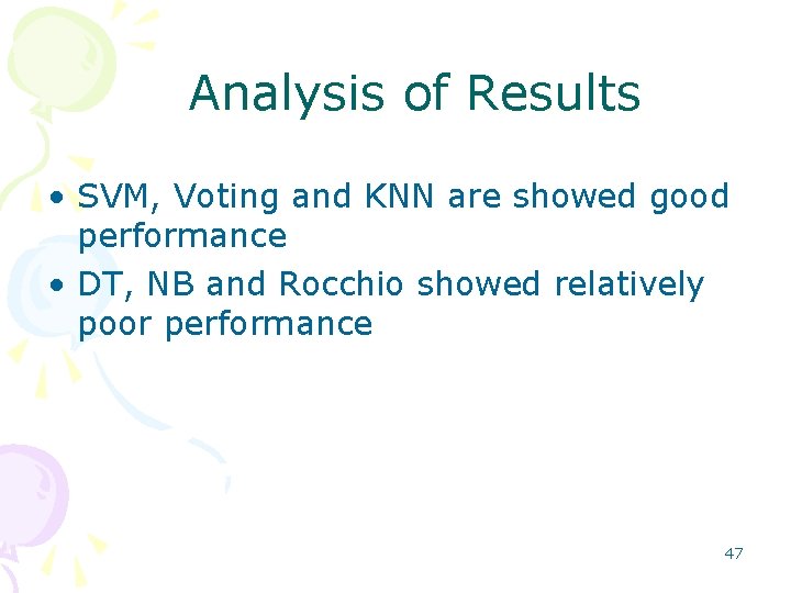
Analysis of Results • SVM, Voting and KNN are showed good performance • DT, NB and Rocchio showed relatively poor performance 47

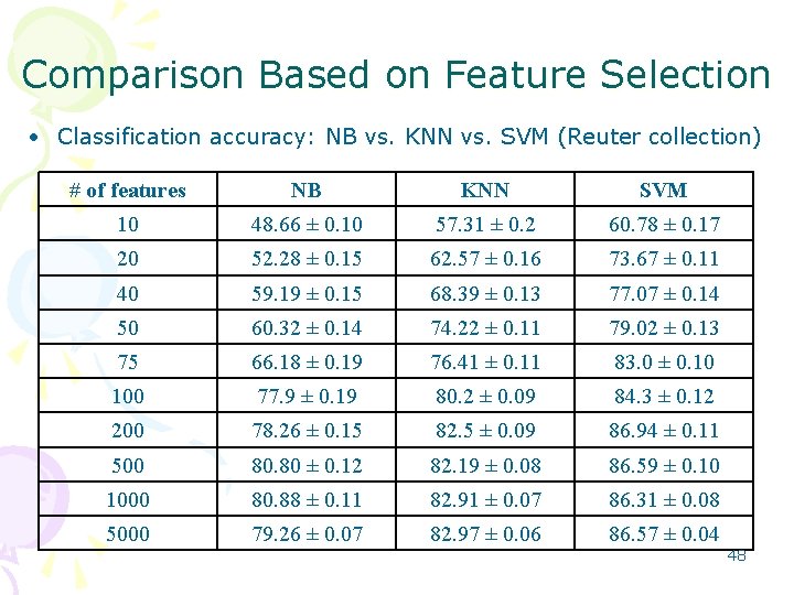
Comparison Based on Feature Selection • Classification accuracy: NB vs. KNN vs. SVM (Reuter collection) # of features NB KNN SVM 10 48. 66 ± 0. 10 57. 31 ± 0. 2 60. 78 ± 0. 17 20 52. 28 ± 0. 15 62. 57 ± 0. 16 73. 67 ± 0. 11 40 59. 19 ± 0. 15 68. 39 ± 0. 13 77. 07 ± 0. 14 50 60. 32 ± 0. 14 74. 22 ± 0. 11 79. 02 ± 0. 13 75 66. 18 ± 0. 19 76. 41 ± 0. 11 83. 0 ± 0. 10 100 77. 9 ± 0. 19 80. 2 ± 0. 09 84. 3 ± 0. 12 200 78. 26 ± 0. 15 82. 5 ± 0. 09 86. 94 ± 0. 11 500 80. 80 ± 0. 12 82. 19 ± 0. 08 86. 59 ± 0. 10 1000 80. 88 ± 0. 11 82. 91 ± 0. 07 86. 31 ± 0. 08 5000 79. 26 ± 0. 07 82. 97 ± 0. 06 86. 57 ± 0. 04 48

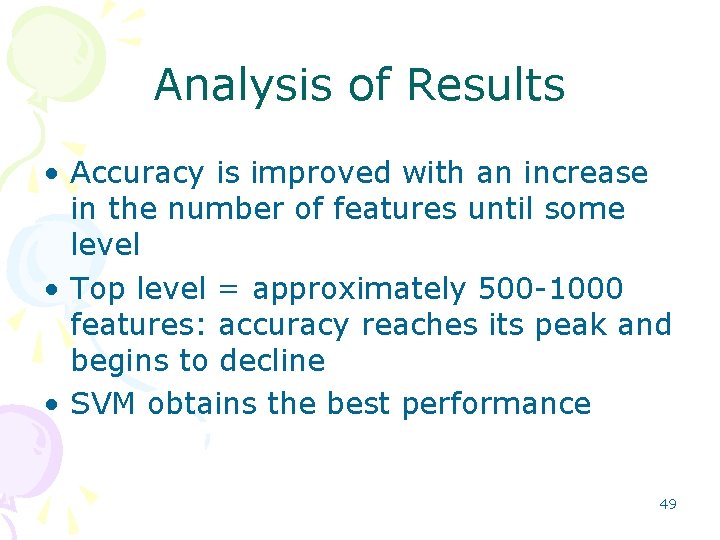
Analysis of Results • Accuracy is improved with an increase in the number of features until some level • Top level = approximately 500 1000 features: accuracy reaches its peak and begins to decline • SVM obtains the best performance 49

Conclusion • Different algorithms perform differently depending on data collections • Some algorithms (e. g. Rocchio) do not perform well • None of them appears to be globally superior over the others; however, SVM and Voting are good choices by considering all the factors 50