IE 607 Heuristic Optimization Introduction to Optimization 1

IE 607 Heuristic Optimization Introduction to Optimization 1

• Objective Function Max (Min) some function of decision variables Subject to (s. t. ) equality (=) constraints inequality ( ) constraints • Search Space Range or values of decisions variables that will be searched during optimization. Often a calculable size in combinatorial optimization 2

Types of Solutions • A solution to an optimization problem specifies the values of the decision variables, and therefore also the value of the objective function. • A feasible solution satisfies all constraints. • An optimal solution is feasible and provides the best objective function value. • A near-optimal solution is feasible and provides a superior objective function value, but not necessarily the best. 3

Continuous vs Combinatorial • Optimization problems can be continuous (an infinite number of feasible solutions) or combinatorial (a finite number of feasible solutions). • Continuous problem generally maximize or minimize a function of continuous variables such as min 4 x + 5 y where x and y are real numbers • Combinatorial problems generally maximize or minimize a function of discrete variables such as min 4 x + 5 y where x and y are countable items (e. g. integer only). 4

Definition of Combinatorial Optimization • Combinatorial optimization is the mathematical study of finding an optimal arrangement, grouping, ordering, or selection of discrete objects usually finite in numbers. - Lawler, 1976 • In practice, combinatorial problems are often more difficult because there is no derivative information and the surfaces are not smooth. 5

Constraints • Constraints can be hard (must be satisfied) or soft (is desirable to satisfy). Example: In your course schedule a hard constraint is that no classes overlap. A soft constraint is that no class be before 10 AM. • Constraints can be explicit (stated in the problem) or implicit (obvious to the problem). 6

• TSP (Traveling Salesman Problem) Given the coordinates of n cities, find the shortest closed tour which visits each once and only once (i. e. exactly once). Example: In the TSP, an implicit constraint is that all cities be visited once and only once. 7

Aspects of an Optimization Problem • Continuous or Combinatorial • Size – number of decision variables, range/count of possible values of decision variables, search space size • Degree of constraints – number of constraints, difficulty of satisfying constraints, proportion of feasible solutions to search space • Single or Multiple objectives 8

Aspects of an Optimization Problem • Deterministic (all variables are deterministic) or Stochastic (the objective function and/or some decision variables and/or some constraints are random variables) • Decomposition – decomposite a problem into series problems, and then solve them independently • Relaxation – solve problem beyond relaxation, and then can solve it back easier 9

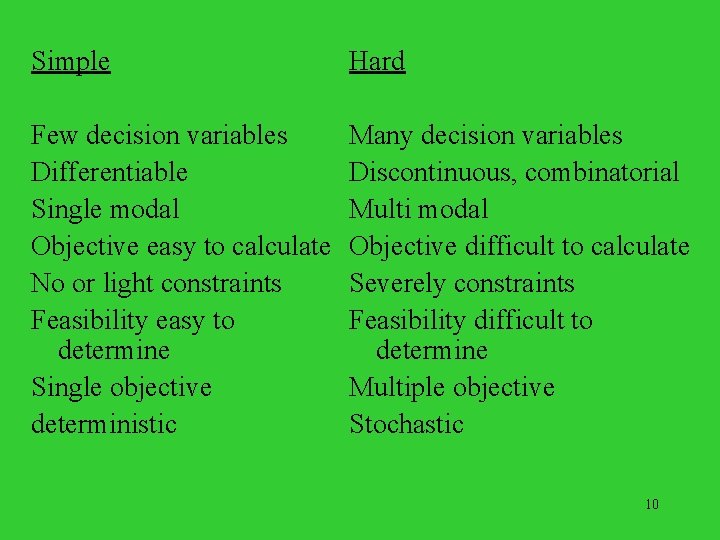
Simple Hard Few decision variables Differentiable Single modal Objective easy to calculate No or light constraints Feasibility easy to determine Single objective deterministic Many decision variables Discontinuous, combinatorial Multi modal Objective difficult to calculate Severely constraints Feasibility difficult to determine Multiple objective Stochastic 10

• For Simple problems, enumeration or exact methods such as differentiation or mathematical programming or branch and bound will work best. • For Hard problems, differentiation is not possible and enumeration and other exact methods such as math programming are not computationally practical. For these, heuristics are used. 11

Search Basics • Search is the term used for constructing/improving solutions to obtain the optimum or near-optimum. Solution Encoding (representing the solution) Neighborhood Move Nearby solutions (in the encoding or solution space) Transforming current solution to another (usually neighboring) solution Evaluation The solutions’ feasibility and objective 12 function value

• Constructive search techniques work by constructing a solution step by step, evaluating that solution for (a) feasibility and (b) objective function. • Improvement search techniques work by constructing a solution, moving to a neighboring solution, evaluating that solution for (a) feasibility and (b) objective function. 13

• Search techniques may be deterministic (always arrive at the same final solution through the same sequence of solutions, although they may depend on the initial solution). Examples are LP (simplex method), tabu search, simple heuristics like FIFO, LIFO, and greedy heuristics. • Search techniques may be stochastic where the solutions considered and their order are different depending on random variables. Examples are simulated annealing, ant colony optimization and genetic algorithms. 14

• Search techniques may be local, that is, they find the nearest optimum which may not be the real optimum. Example: greedy heuristic (local optimizers). • Search techniques may be global, that is, they find the true optimum even if it involves moving to worst solutions during search (nongreedy). 15

Heuristics • Heuristics are rules to search to find optimal or near-optimal solutions. Examples are FIFO, LIFO, earliest due date first, largest processing time first, shortest distance first, etc. • Heuristics can be constructive (build a solution piece by piece) or improvement (take a solution and alter it to find a better solution). 16

• Many constructive heuristics are greedy or myopic, that is, they take the best thing next without regard for the rest of the solution. Example: A constructive heuristic for TSP is to take the nearest city next. An improvement heuristic for TSP is to take a tour and swap the order of two cities. 17

Meta-Heuristics An iterative generation process which guides a subordinate heuristic by combining intelligently different concepts derived from classical heuristics, artificial intelligence, biological evolution, natural and physical sciences for exploring and exploiting the search spaces using learning strategies to structure information in order to find efficiently near-optimal solutions. - Osman and Kelly, 1996 18

• • • This course will focus on meta-heuristics inspired by nature. Meta-heuristics are not tied to any special problem type and are general methods that can be altered to fit the specific problem. The inspiration from nature is: Simulated Annealing (SA) – molecule/crystal arrangement during cool down Evolutionary Computation (EC) – biological evolution Tabu Search (TS) – long and short term memory Ant Colony and Swarms - individual and group behavior using communication between agents 19

Advantages of Meta-Heuristics • Very flexible • Often global optimizers • Often robust to problem size, problem instance and random variables • May be only practical alternative 20

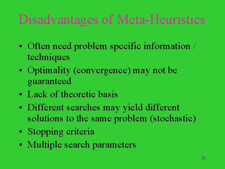
Disadvantages of Meta-Heuristics • Often need problem specific information / techniques • Optimality (convergence) may not be guaranteed • Lack of theoretic basis • Different searches may yield different solutions to the same problem (stochastic) • Stopping criteria • Multiple search parameters 21

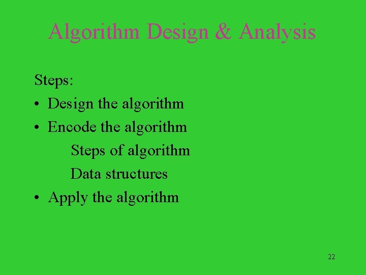
Algorithm Design & Analysis Steps: • Design the algorithm • Encode the algorithm Steps of algorithm Data structures • Apply the algorithm 22

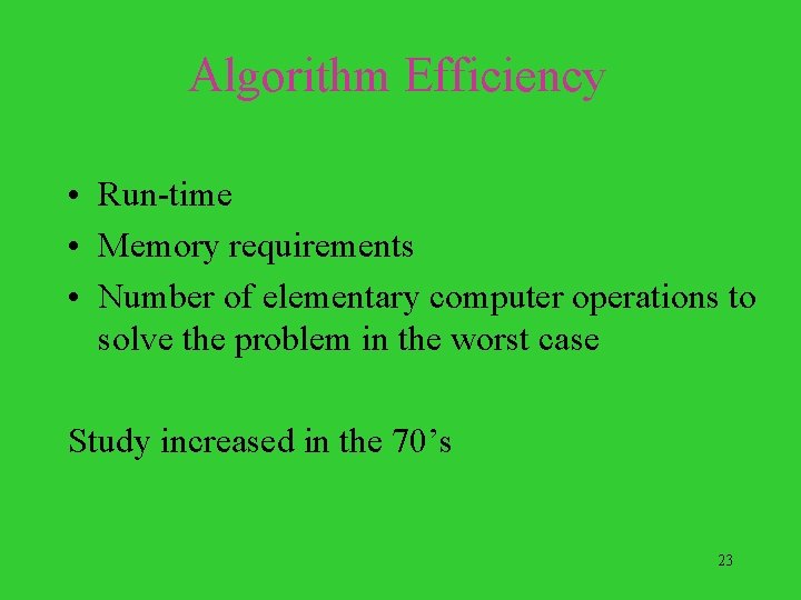
Algorithm Efficiency • Run-time • Memory requirements • Number of elementary computer operations to solve the problem in the worst case Study increased in the 70’s 23

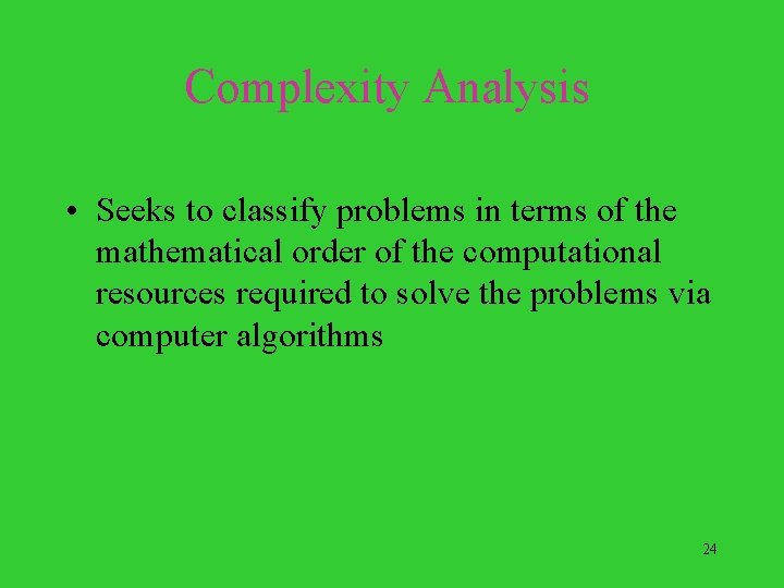
Complexity Analysis • Seeks to classify problems in terms of the mathematical order of the computational resources required to solve the problems via computer algorithms 24

• Problem is a collection of instances that share a mathematical form but differ in size and in the values of numerical constants in the problem form (i. e. generic model) Example: shortest path. • Instance is a special case of problem with specified data and parameters. • An algorithm solves a problem if the algorithm is guaranteed to find the optimal solution for any instance. 25

Complexity Measures • Empirical Analysis - see how algorithms perform in practice - write program, test on classes of problem instances • Average Case Analysis - determine expected number of steps - choose probability distribution for problem instances, use statistical analysis to derive asymptotic expected run times 26

Complexity Measures • Worst Case Analysis - provides upper bound (UB) on the number of steps an algorithm can take on any instance - count largest possible number of steps - provides a “guarantee” on number of steps the algorithm will need 27

Complexity Measures • CONs of Empirical Analysis - algorithm performance depends on computer language, compiler, hardware, programmer’s skills - costly and time consuming to do - algorithm comparison can be inconclusive 28

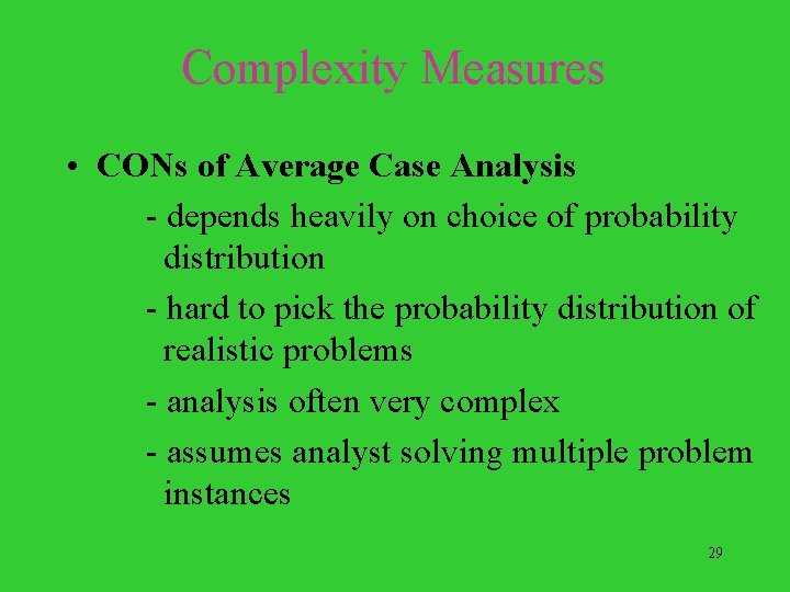
Complexity Measures • CONs of Average Case Analysis - depends heavily on choice of probability distribution - hard to pick the probability distribution of realistic problems - analysis often very complex - assumes analyst solving multiple problem instances 29

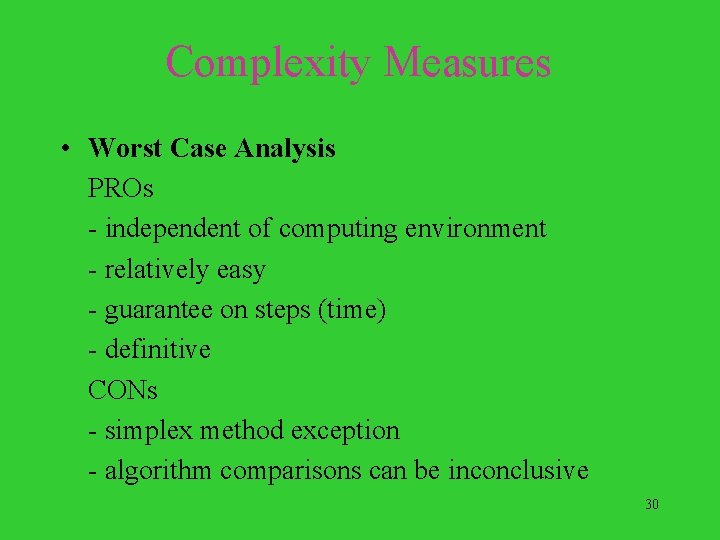
Complexity Measures • Worst Case Analysis PROs - independent of computing environment - relatively easy - guarantee on steps (time) - definitive CONs - simplex method exception - algorithm comparisons can be inconclusive 30

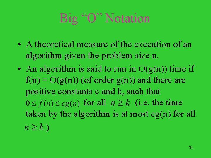
Big “O” Notation • A theoretical measure of the execution of an algorithm given the problem size n. • An algorithm is said to run in O(g(n)) time if f(n) = O(g(n)) (of order g(n)) and there are positive constants c and k, such that for all (i. e. the time taken by the algorithm is at most cg(n) for all ) 31

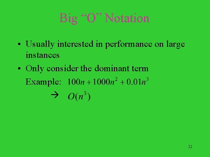
Big “O” Notation • Usually interested in performance on large instances • Only consider the dominant term Example: 32

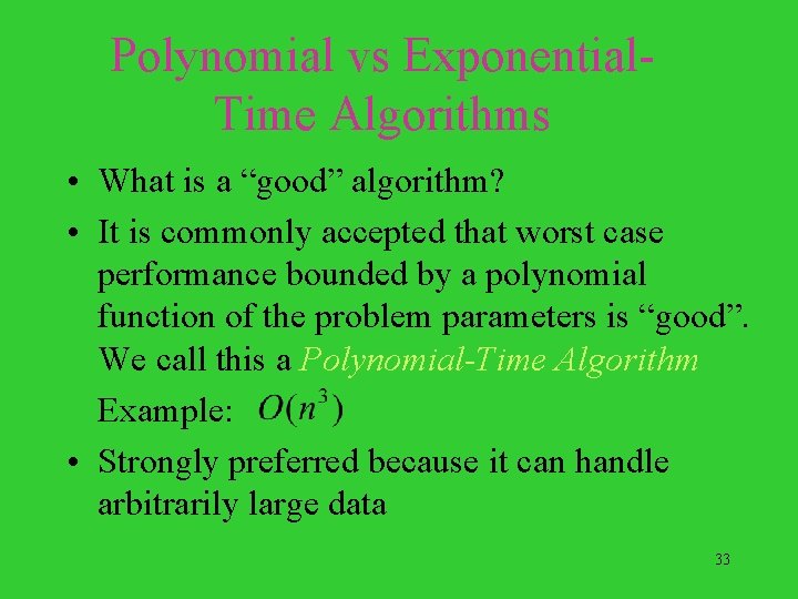
Polynomial vs Exponential. Time Algorithms • What is a “good” algorithm? • It is commonly accepted that worst case performance bounded by a polynomial function of the problem parameters is “good”. We call this a Polynomial-Time Algorithm Example: • Strongly preferred because it can handle arbitrarily large data 33

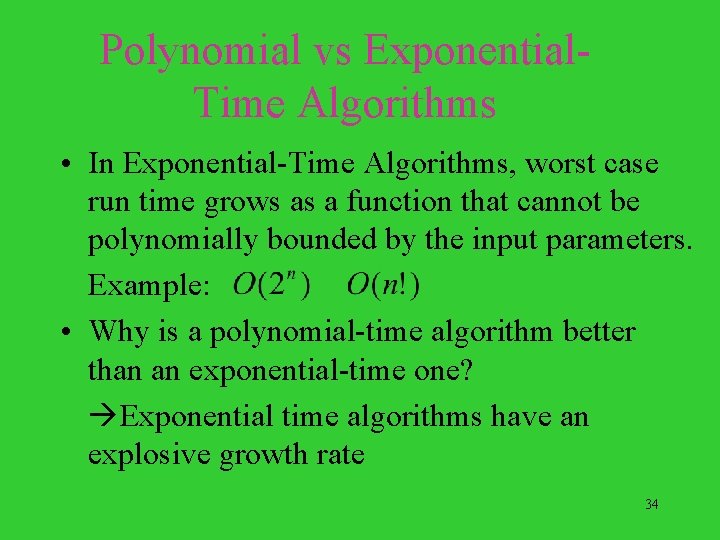
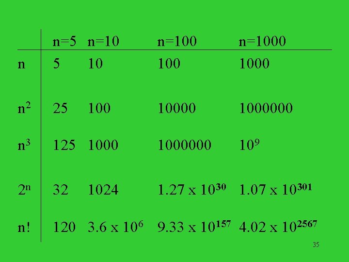
Polynomial vs Exponential. Time Algorithms • In Exponential-Time Algorithms, worst case run time grows as a function that cannot be polynomially bounded by the input parameters. Example: • Why is a polynomial-time algorithm better than an exponential-time one? Exponential time algorithms have an explosive growth rate 34

n n=5 n=10 5 10 n=1000 n 2 25 1000000 n 3 125 1000000 109 2 n 32 1. 27 x 1030 1. 07 x 10301 n! 120 3. 6 x 106 9. 33 x 10157 4. 02 x 102567 100 1024 35

Optimization vs Decision Problems • Optimization Problem A computational problem in which the object is to find the best of all possible solutions. (i. e. find a solution in the feasible region which has the minimum or maximum value of the objective function. ) • Decision Problem A problem with a “yes” or “no” answer. 36

• Convert Optimization Problems into equivalent Decision Problems What is the optimal value? Is there a feasible solution to the problem with an objective function value equal to or superior to a specified threshold? 37

Class P • The class of decision problems for which we can find a solution in polynomial time. i. e. P includes all decision problems for which there is an algorithm that halts with the correct yes/no answer in a number of steps bounded by a polynomial in the problem size n. • The Class P in general is thought of as being composed of relatively “easy” problems for which efficient algorithms exist. 38

Examples of Class P Problems • • • Shortest path Minimum spanning tree Network flow Transportation, assignment and transshipment Some single machine scheduling problems 39

Class NP • NP = Nondeterministic Polynomial • NP is the class of decision problems for which we can check solutions in polynomial time. i. e. easy to verify but not necessarily easy to solve 40

Class NP • Formally, it is the set of decision problems such that if x is a “yes” instance then this could be verified in polynomial time if a clue or certificate whose size is polynomial in the size of x is appended to the problem input. • NP includes all those decision problems that could be polynomial-time solved if the right (polynomial-length) clue is appended to the problem input. 41

Class P vs Class NP • Class P contains all those that have been conquered with well-bounded, constructive algorithms. • Class NP includes the decision problem versions of virtually all the widely studied combinatorial optimization problems. • P is a subset of NP. 42

Polynomial Reduction • Problem P reduces in polynomial-time to another problem P´, if and only if, - there is an algorithm for problem P which uses problem P´ as a subroutine, - each call to the subroutine of problem P´ counts as a single step, - this algorithm for problem P´ runs in polynomial-time. 43

Polynomial Reduction • If problem P polynomially reduces to problem P´ and there is a polynomial-time algorithm for problem P´, then there is a polynomial-time algorithm for problem P. Problem P´ is at least as hard as problem P! 44

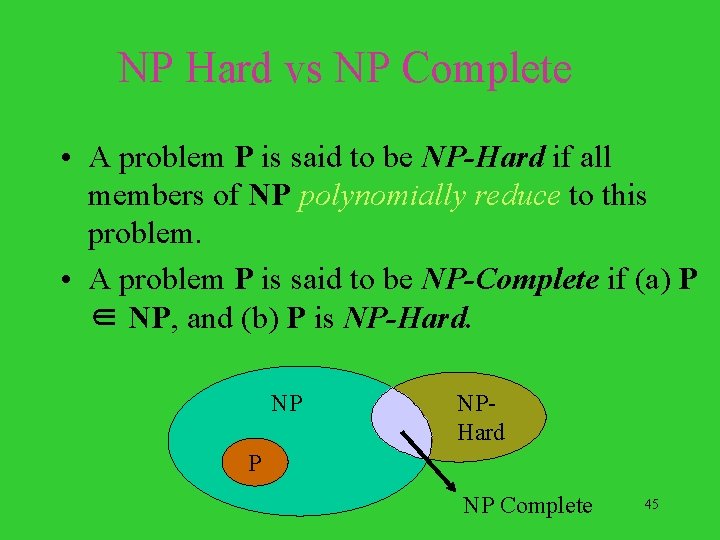
NP Hard vs NP Complete • A problem P is said to be NP-Hard if all members of NP polynomially reduce to this problem. • A problem P is said to be NP-Complete if (a) P ∈ NP, and (b) P is NP-Hard. NP NPHard P NP Complete 45

• If there is an efficient (i. e. polynomial) algorithm for some NP-Complete problem, then there is a polynomial algorithm existing for all problems in NP. P = NP • Examples of NP-Hard problems: TSP, graph coloring, set covering and partitioning, knapsack, precedence-constrained scheduling, etc. 46