IDL 102 Particle Tracking Our MO Convert Image
")

 •")
 •")
 •")


")
")
")


")
 4 2 t=1 7 9 13 10 6 5")
 2 t=1 7 9 13 10 6 5 3")
 2 t=1 7 9 13 10 6 5 3")
 mx x m= D 1")
")
")
 Constant velocity gives a slope 2 on a log-log")


- Slides: 45
IDL 102 (Particle Tracking)
Our MO • Convert Image DV -> gdf – Do not byte-scale – Also, do byte scale (after conversion) • Find dots in each frame – “Clean” image – Find all candidate dots – Refine dots set • Link dots frame-to-frame to get trajectories – How far are we willing to look for a particle? – How about gaps? – How about blinky, random noise?
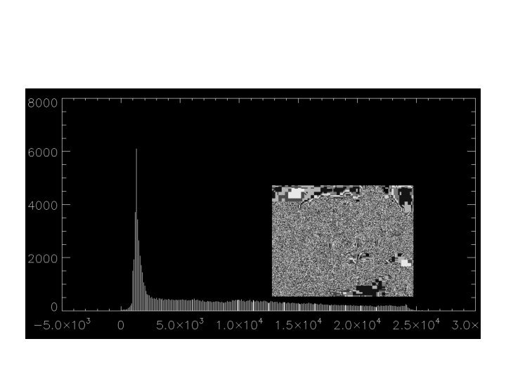
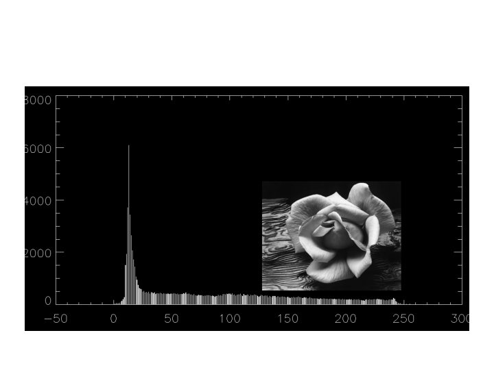
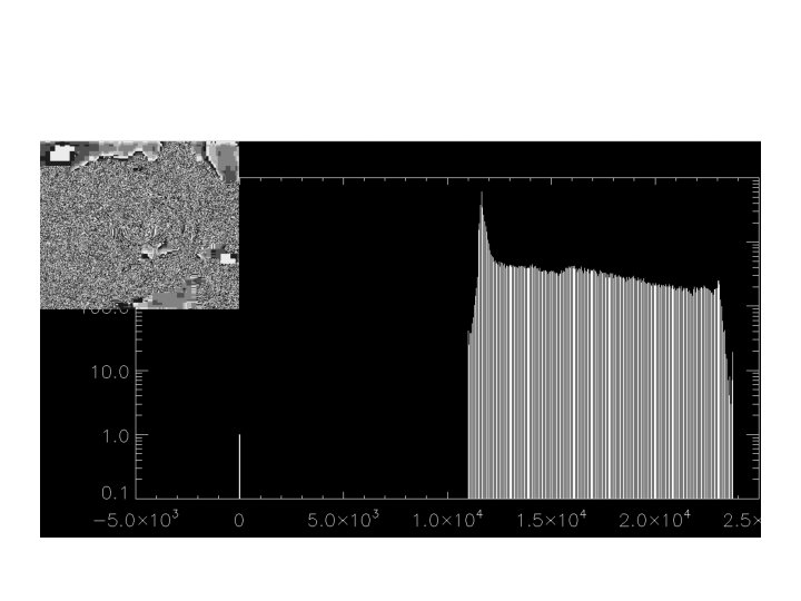
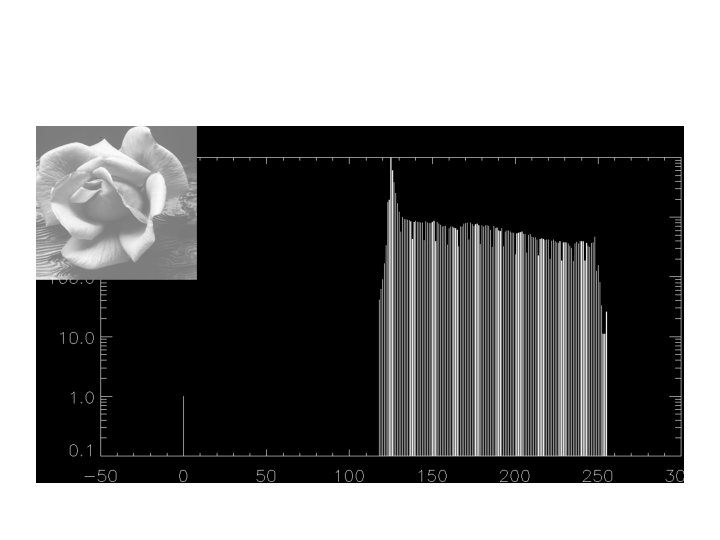
Conversion isn’t futile • Images are acquired at 16 bit (0 -> 216=65536) • Images have to be displayed at 8 bit (0 -> 28=256)
Conversion isn’t futile • Images are acquired at 16 bit (0 -> 216=65536) • Images have to be displayed at 8 bit (0 -> 28=256)
Conversion isn’t futile • Images are acquired at 16 bit (0 -> 216=65536) • Images have to be displayed at 8 bit (0 -> 28=256)
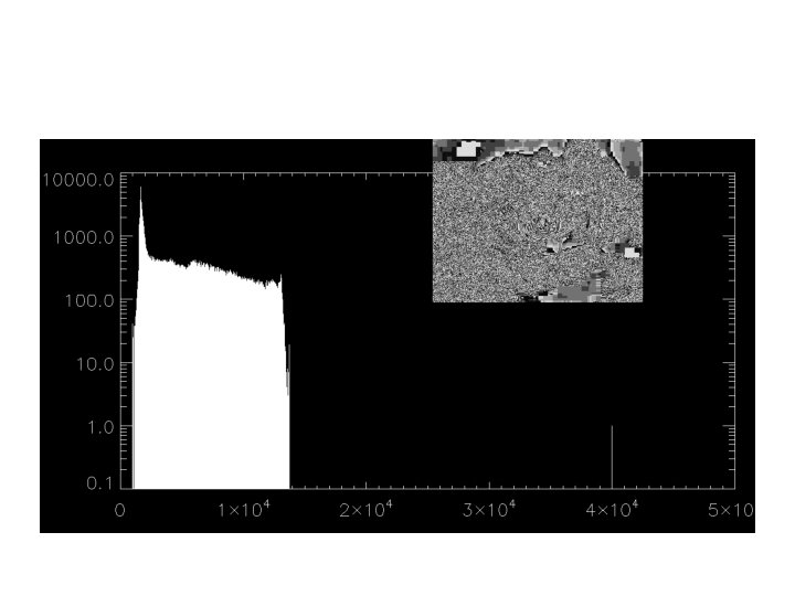
HOT pixels are bad
HOT pixels are bad
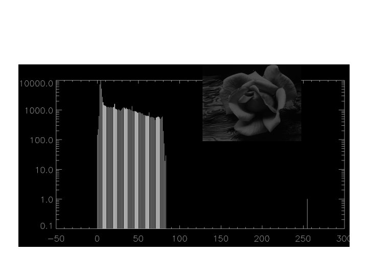
DEAD pixels are bad too
DEAD pixels are bad too
Pre-tracking • Find dots in each frame – “Clean” image – Find all candidate dots – Refine dots set
Cleaning the image: band-passing with bpass. pro
Cleaning the image: band-passing with bpass. pro
Cleaning the image: band-passing with bpass. pro
Cleaning the image: band-passing with bpass. pro
Cleaning the image: band-passing with bpass. pro
Cleaning the image: band-passing with bpass. pro
These could be candidates
Select them with a reasonable masscut
You need to refine them using reasonable criteria X 0 1 2 3 4 5 6 7 8 9 10 11 12 13 14 0 3 8 13 18 23 28 33 38 43 48 53 58 63 68 73 Y Mass 1 2 3 4 5 6 7 0 9 10 11 12 0 14 15 16 17 0 19 20 21 22 0 24 25 26 27 2 29 30 31 32 2 34 35 36 37 3 39 40 41 42 4 44 45 46 47 5 49 50 51 52 5 54 55 56 57 5 59 60 61 62 5 64 65 66 67 6 69 70 71 72 12 74 75 76 77 12 Radius Eccentricity Time
Criteria • X, Y can be used to clip edges, where things usually go wrong • “Mass” is total integrated brightness in each blob • Radius of gyration is a measure of size that makes dimmer pixels count less • Eccentricity: – 0: a perfect disk – 1: a perfect line segment • Use eclip. pro, where(), or edgeclip. pro to refine ranges of these criteria
A few things you can use to evaluate your pretracking: • Say your pretracked data is in ‘pt’ • Overview: – ptexplore, pt • Number of particles at each frame (bleaching? ) – plot_hist, pt[5, *], bin=1 • Bias towards integer pixel positions – plot_hist, pt[0: 1, *] mod 1, bin=. 05
Now track them! • User defined params for tracking: – Distance to look for same particle frame-toframe • This must me less than interparticle distance in each frame – Number of frames a particle is allowed to disappear • This must be less than time it takes for two particles to switch position – Shortest trajectory you consider real • This is a toughie. But setting this to something >0 helps get rid of artifacts that blink
Check tracking with • P(dx, dt=1)
Check tracking with • P(dx, dt=1)
Check tracking with • P(dx, dt=1)
Check with IDover 2 D
Analysis
Analyze Mean squared displacement (MSD)
Analyze Mean squared displacement (MSD) 4 2 t=1 7 9 13 10 6 5 3 11 8 12 15 14
Analyze Mean squared displacement (MSD) 2 t=1 7 9 13 10 6 5 3 11 12 8 • Measure all displacements that are Dt = 1 frame apart • Square them • Average over other particles if desired and “allowed” 15 14 MSD(mm 2) 4 1 13 Dt (frames)
Analyze Mean squared displacement (MSD) 2 t=1 7 9 13 10 6 5 3 11 12 8 • Measure all displacements that are Dt = 1 frame apart • Square them • Average over other particles if desired and “allowed” • Then do it for Dt = 2 frames and so on 15 14 MSD(mm 2) 4 12 13 Dt (frames)
Says Einstein! constant in biology y = MSD(mm 2) mx x m= D 1 m= D 2 Dt (frames)
A Yes/No test for diffusion (What’s this about logs and slopes of 1? )
A Yes/No test for diffusion (What’s this about logs and slopes of 1? ) 1 1 y = c m +x x 2
Ballistic motion (that of projectiles) Constant velocity gives a slope 2 on a log-log plot
What about this mess of an MSD plot?
What about this mess of an MSD plot?
What about this mess of an MSD plot?
What about this mess of an MSD plot?