Ice sheet and glacier modeling Kernel of the

Ice sheet and glacier modeling

Kernel of the ice sheet model • Thermomechanically coupled ice flow and dynamics model: – mass, force and angular momentum balance – Energy balance equation – Ice thickness equation

Hierarchy of approximations • Ice flow is quasi-stationary – very fast reaction, very short transition time – temporal changes in ice flow do not correspond to the Euler acceleration • The system is shallow – vertical extent generally much smaller than horizontal extent – vertical component of velocity generally much smaller than horizontal component – nearly lithostatic flow • Negligible processes: – Coriolis force, no convection, no turbulence • Difficulties: – – Non-Newtonian, sometimes anisotropic flow properties Compressible firn areas Polythermal conditions with englacial phase boundaries Discontinuities such as fracturing, hydraulic system, sliding

Stokes force balance

Hydrostatic force balance

From definition of deviatoric stress tensor: Substitute in stress divergence: hydrostatic stress equation

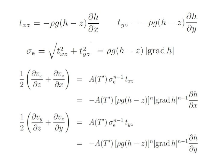
Glen’s flow law in components: Because of the incompressibility, only 2 of the 3 equations on left side are independent

Hydrostatic approximation Substitution of the components of Glen’s flow law in the hydrostatic stress equation yields

Omitting 2 nd-order terms yiels the so called first order approximation Vertical velocity component uncoupled from Horizontal velocity components

Omitting first order terms yields the shallow ice approximation Only z-derivatives: velocity field only depends on the local conditions (surface inclination, ice thickness

Scales • shallowness: geometric aspect ratio small – defines scaling parameter for hierarchy of approximations • the “process aspect ratio” may be locally much larger – horizontal gradients of field variables may be large due to locally steep topography or transitions • “numerical grid aspect ratio” – horizontal grid resolution compared with mean ice thickness (or vertical grid resolution) • what means “the approximation is accurate to a given order e. g. in the aspect ratio? ” – usually this refers to the predictability of the evolution of the overall volume of the ice mass – this can not refer to the accuracy of the prediction of local patterns in the fields – Predictive power questionable

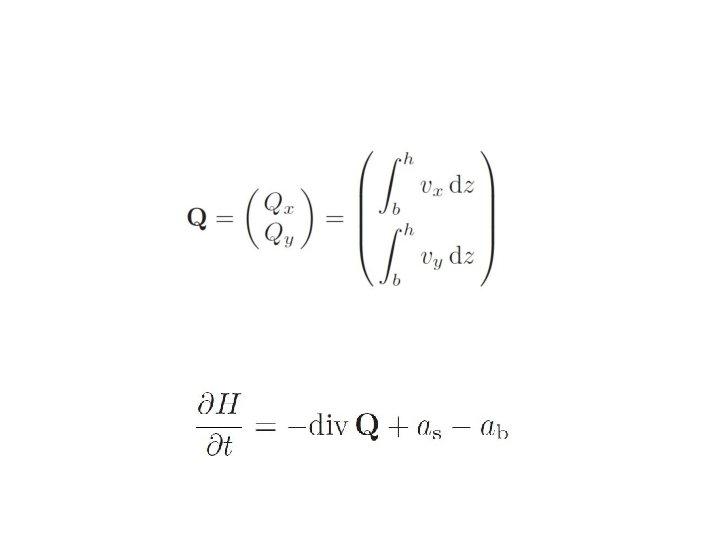
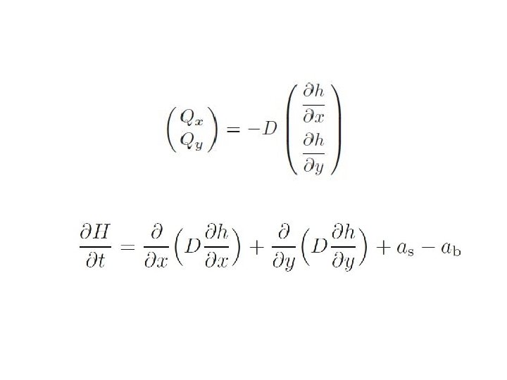
Shallow ice approximation • Treats the ice sheet locally like a parallel sided slab: – Velocity profile depends only on local quantities: surface inclination, ice thickness and vertical temperature profile (no horizontal coupling) – Differential equation for horizontal ice velocity can be reduced to quadrature (integral along vertical profile) – Vertical component of velocity can be obtained by integration of mass continuity along vertical profile

Integration of velocity components:

The horizontal velocity vector always points In the direction of the steepest surface slope

With the basal shear stress we obtain the basal (sliding) velocity

Shallow thermodynamics

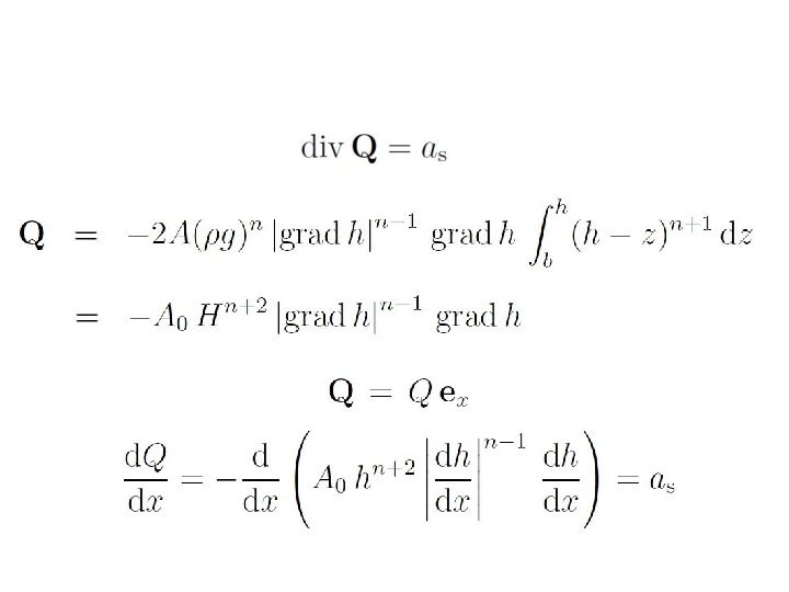
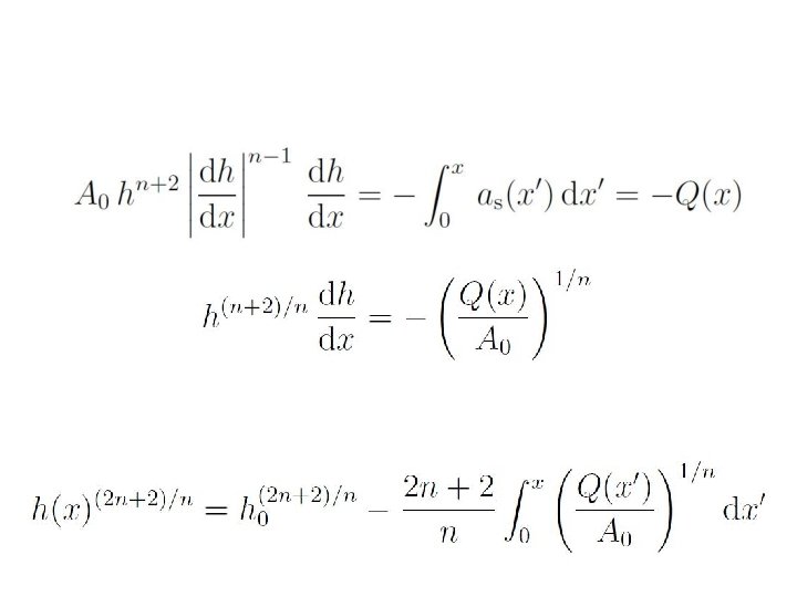
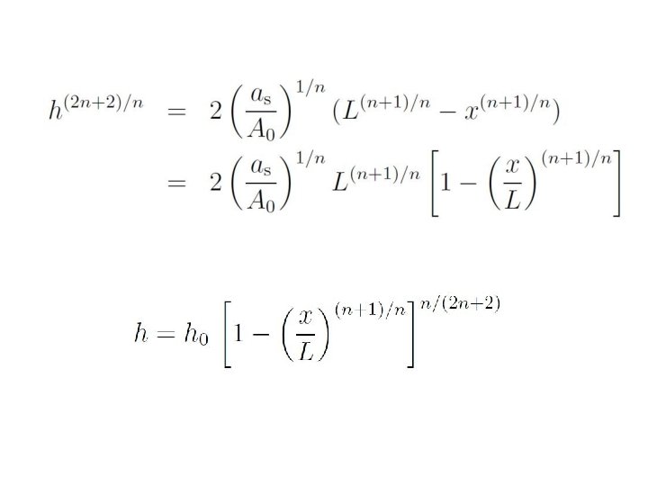
Exact solutions of the ice sheet equation

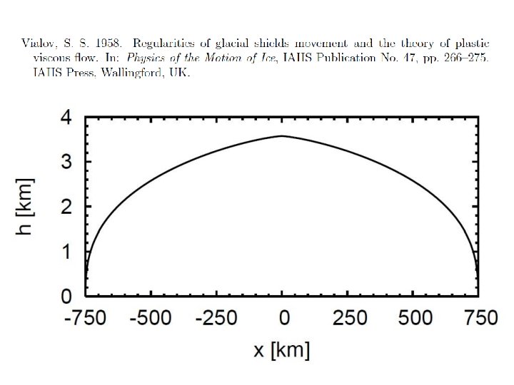
Vialov profile

Consequences of shallowness: Horizontal ice flux in a slab is proportional to the Ice thickness to the n+2 power (if n=3, 5 th power) Vertical velocity component equals the horizontal flux divergence

The relative error in the horizontal velocity component Relates the errors in the ice thickness and inclination The absolute error in the vertical component relates to the error in the horizontal component The relative error in the vertical velocity component is

Modelled vs. remotely measured mass balance: scatter in the modelled vertical velocity component Arolla glacier

Shallowness • Little coupling in horizontal direction – Critical for transitions: sliding-non sliding, grounded-floating, shearing-streaming – Coupling only through mass continuity: vertical velocity component – Critical for vertical energy advection and resulting temperature profiles • Vertical flow component reacts very sensititive to changes in the horizontal flow component: – High resolution: N very large, digit eliminination – Low resolution: right side fraction inaccuarate – Relative error in the vertical component is large compared to the relative error in the horizontal component

temporal scales • Mass balance time scale: – defined by the mean climatic mass flux at the surface of the ice mass, e. g. fraction of mean ice thickness and mean mass balance – decades for alpine glaciers, centuries for ice caps, millenia for ice sheets – different for growth and shrinking of ice masses • Event or catastrophe time scales: – unstable glacier retreat, unstable calving, unstable grounding line, surges, streaming – years to centuries? ? ? for unstable calving, grounding lines of glaciers or ice sheets – months to decades (centuries? ) for surges – irreversibility? point of no return?

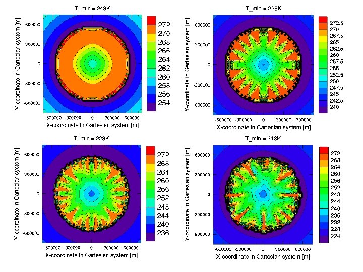
Condition of the system • Coupled system of non-linear equations on all levels of approximations – Stability and accuracy of discretised system • Shallowness makes it “ill-conditioned” – Error amplification (vertical components) – Boundaries must be constrained on both sides (bad inversion) • Requires verification (and intercomparison? ) • What are the reasons for the spokes in the EISMINT intercomparison experiments? – Physics versus mathematics versus numerics?

First order approximation Aspect ratio

Scaling with the aspect ratio e Aspect ratio Horizontal and vertical extents: [H] and [L] Typical corresponding velocity components: [U] and [W]

Scaling Only keep terms in the equationof which the order of magnitude is O(1) or O(e) but omit Terms of O(e 2) and smaller. In 2 -dimensions: Remaining stress terms are

First order equations written in stress terms t. Dxx: longitudinal deviatoric stress txz: shear stress v x: longitudinal velocity component h: r: g: x, z: viscosity ice thickness ice density gravity longitudinal and vertical coordinates

First order equations with velocity

Arolla glacier: first order (FOA) vs. shallow ice approximation (SIA)

Fixed point shooting scheme Exercise given in Problemsheets and Programs to download from my ftp site

Transformed equations Equations suitable for the method of lines: can be transformed into 2 first order differential equations And one algebraic equation (discretisation)

Discretised equations

Shooting scheme with line integration: surface shear Traction must be zero Fixed point iteration: Chose basal shear traction, integrate along vertical Lines to the surface and test if the surface traction is zero If not: new basal traction and repeat until convergence

First order vs shallow ice approximation • First order and shallow ice approximation are very different: not only small perturbation • Difference between FOA and SIA of same order of magnitude • Basal sliding in FOA feeds back to entire stress field, not in SIA • FOA smoothes out variations in the horizontal dierections (can flow across bump or through depression, sliding non-sliding transitions) • Strongly limits application of SIA

Basal boundary condition • Sliding parameterization – bad knowledge on basal conditions – bad knowledge for quantification of physical processes related to sliding • Sliding implementation – sliding is not locally defined – sliding / non sliding transitions

Sliding implementation in higher order models • basal layer: power law rheology defines power law sliding parameterization • membrane stresses handled by higher order flow model • basal layer can, but does not need to have physical meaning (implementation)

Full Stokes models • All velocity components are coupled • Heat diffusion considered in all directions • Mostly use finite element methods on unstructured grids, which is suitable for irregular geometries • Computationally expensive • Existing models: ELMER Ice, EPFL Model etc.

EPFL Model (Jouvet, 2010) • 3 D Full Stokes flow: unstructured finite element mesh • volume of fluid: uniform Cartesian grid • coupled mass balance: Hock model