ICAO Strategic Objective Economic Development of Air Transport

ICAO Strategic Objective: Economic Development of Air Transport Introduction to Forecasting Analysis ICAO Aviation Data Analyses Seminar Middle East (MID) Regional Office 27 -29 October Economic Analysis and Policy (EAP) Section Air Transport Bureau (ATB)

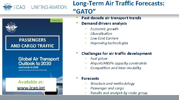
Long-Term Air Traffic Forecasts: “GATO” • • PASSENGERS AND CARGO TRAFFIC Available at: www. icao. int Past decade air transport trends Demand drivers analysis - Economic growth Liberalization Low Cost Carriers Improving technologies • Challenges for air traffic development • Forecasts - Fuel prices Airport/ANSPs capacity constraints Competition and inter-modality Structure and methodology Passenger and cargo Results and analysis by route group

Background Assembly Resolution A 38 -14 Appendix C : Forecasting, planning and economic analyses The Assembly: • Requests the Council to prepare and maintain, as necessary, forecasts of future trends and developments in civil aviation of both a general and a specific kind, including, where possible, local and regional as well as global data, and to make these available to Contracting States and support data needs of safety, security, environment and efficiency • Requests the Council to develop one single set of long term traffic forecast, from which customized or more detailed forecasts can be produced for various purposes, such as air navigation systems planning and environmental analysis

Main terms and definitions used in forecasting analysis

Types of Data can be broadly divided into the following three types: - Time series data consist of data that are collected, recorded, or observed over successive increments of time. - Cross-sectional data are observations collected at a single point in time. - Panel data are cross-sectional measurements that are repeated over time, such as yearly passengers carried for a sample of airlines. Of the three types of data, time series data is the most extensively used in traffic forecasts.

Forecasting Timeframe Short-term Forecasts Short-term forecasts generally involve some form of scheduling which may include for example the seasons of the year for planning purposes. The cyclical and seasonal factors are more important in these situations. Such forecasts are usually prepared every 6 months or on a more frequent basis. Some airport operators undertake ‘ultra short term’ forecasts for (e. g. ) the next month in order to provide for specific requirement such as adequate staffing in the peaks.

Forecasting Timeframe Medium-term Forecasts Medium-term forecasts are generally prepared for planning, scheduling, budgeting and resource requirements purposes. The trend factor, as well as the cyclical component, plays a key role in the medium-term forecast as the year to year variations in traffic growth are an important element in the planning process

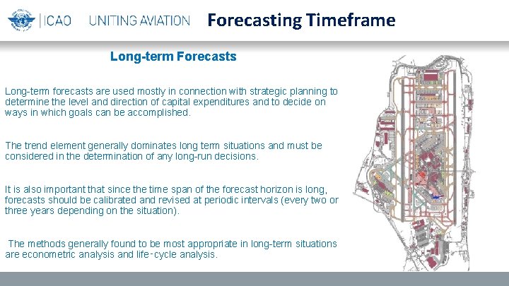
Forecasting Timeframe Long-term Forecasts Long-term forecasts are used mostly in connection with strategic planning to determine the level and direction of capital expenditures and to decide on ways in which goals can be accomplished. The trend element generally dominates long term situations and must be considered in the determination of any long-run decisions. It is also important that since the time span of the forecast horizon is long, forecasts should be calibrated and revised at periodic intervals (every two or three years depending on the situation). The methods generally found to be most appropriate in long-term situations are econometric analysis and life‑cycle analysis.

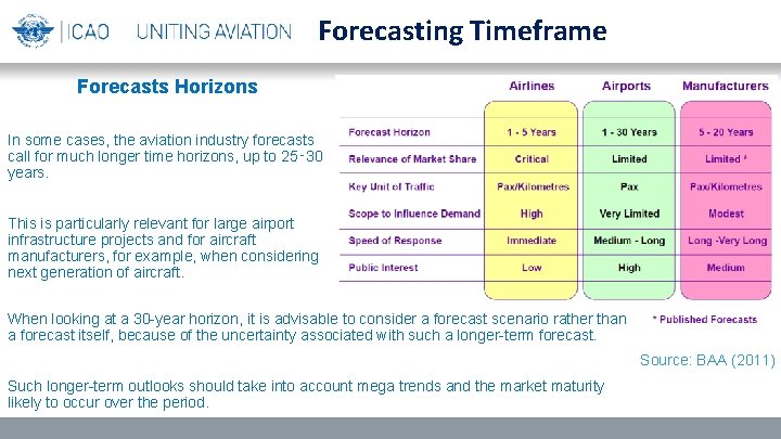
Forecasting Timeframe Forecasts Horizons In some cases, the aviation industry forecasts call for much longer time horizons, up to 25‑ 30 years. This is particularly relevant for large airport infrastructure projects and for aircraft manufacturers, for example, when considering next generation of aircraft. When looking at a 30 -year horizon, it is advisable to consider a forecast scenario rather than a forecast itself, because of the uncertainty associated with such a longer-term forecast. Source: BAA (2011) Such longer-term outlooks should take into account mega trends and the market maturity likely to occur over the period.

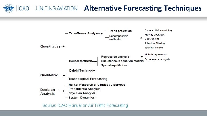
Alternative Forecasting Techniques Source: ICAO Manual on Air Traffic Forecasting

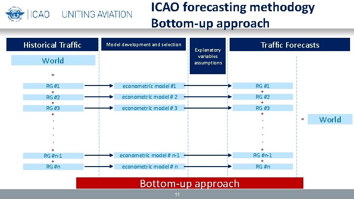
ICAO forecasting methodogy Bottom-up approach Historical Traffic Model development and selection World Explanatory variables assumptions Traffic Forecasts = RG #1 + RG #2 + RG #3 +. . + RG #n-1 + RG #n econometric model #1 econometric model # 2 econometric model # 3 econometric model # n-1 econometric model # n Bottom-up approach 11 RG #1 + RG #2 + RG #3 +. . + RG #n-1 + RG #n = World

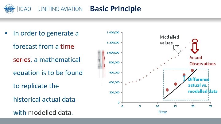
Basic Principle • In order to generate a 1, 400, 000 Modelled values 1, 200, 000 forecast from a time 1, 000 series, a mathematical Actual Observations 800, 000 equation is to be found 600, 000 Difference actual vs. modelled data 400, 000 to replicate the 200, 000 historical actual data with modelled data. 0 0 5 10 15 20 25

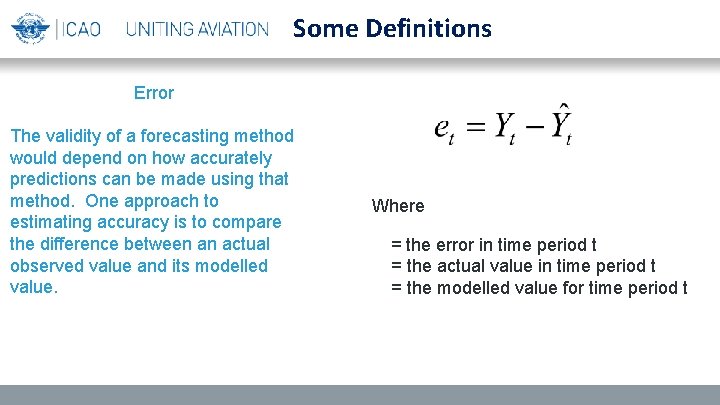
Some Definitions Error The validity of a forecasting method would depend on how accurately predictions can be made using that method. One approach to estimating accuracy is to compare the difference between an actual observed value and its modelled value. Where = the error in time period t = the actual value in time period t = the modelled value for time period t

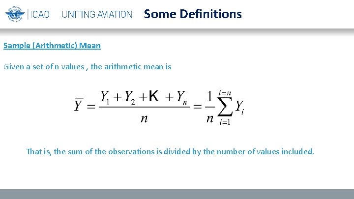
Some Definitions Sample (Arithmetic) Mean Given a set of n values , the arithmetic mean is That is, the sum of the observations is divided by the number of values included.

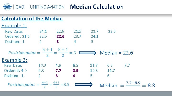
Median Calculation of the Median Example 1: Raw Data: Ordered: 21. 5 Position: 1 24. 1 22. 6 3 21. 5 23. 7 4 23. 7 24. 1 5 Example 2: Raw Data: Ordered: 4. 9 Position: 1 22. 6 Median = 22. 6 10. 3 6. 3 2 4. 9 7. 7 3 8. 9 4 11. 7 10. 3 5 6. 3 11. 7 6 7. 7

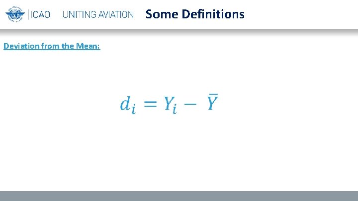
Some Definitions Deviation from the Mean:

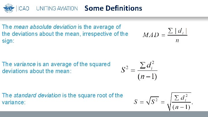
Some Definitions The mean absolute deviation is the average of the deviations about the mean, irrespective of the sign: The variance is an average of the squared deviations about the mean: The standard deviation is the square root of the variance:

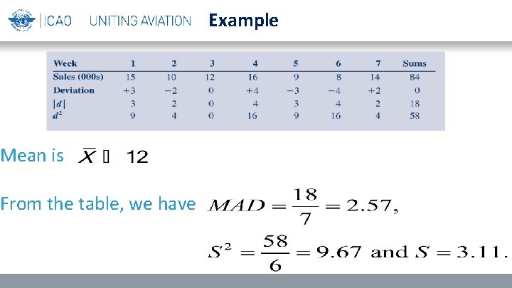
Example Mean is From the table, we have

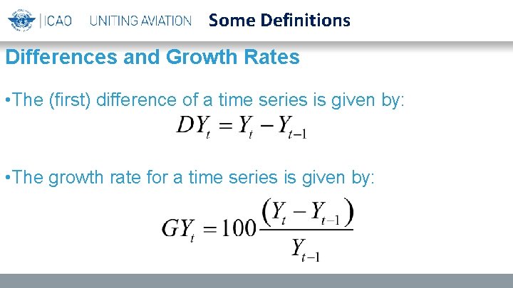
Some Definitions Differences and Growth Rates • The (first) difference of a time series is given by: • The growth rate for a time series is given by:

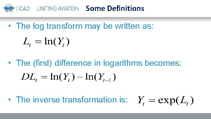
Some Definitions • The log transform may be written as: • The (first) difference in logarithms becomes: • The inverse transformation is:

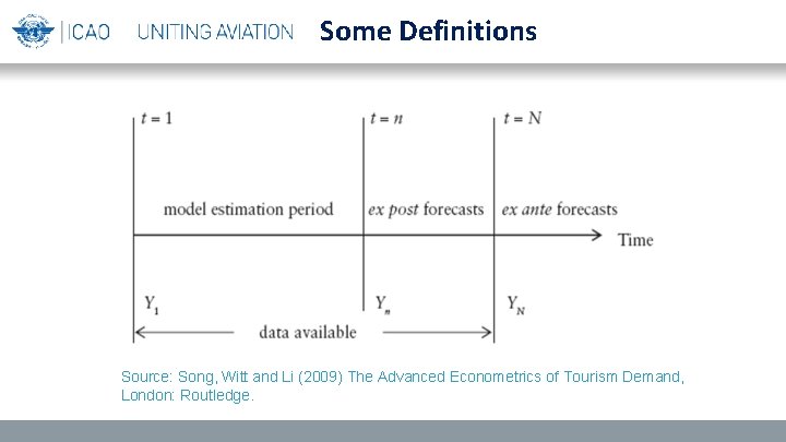
Some Definitions Source: Song, Witt and Li (2009) The Advanced Econometrics of Tourism Demand, London: Routledge.

Practical Example of Time Series Models with Excel

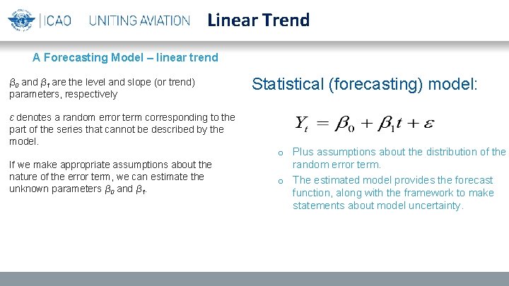
Linear Trend A Forecasting Model – linear trend β 0 and β 1 are the level and slope (or trend) parameters, respectively ε denotes a random error term corresponding to the part of the series that cannot be described by the model. If we make appropriate assumptions about the nature of the error term, we can estimate the unknown parameters β 0 and β 1. Statistical (forecasting) model: o Plus assumptions about the distribution of the random error term. o The estimated model provides the forecast function, along with the framework to make statements about model uncertainty.

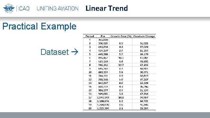
Linear Trend Practical Example Dataset

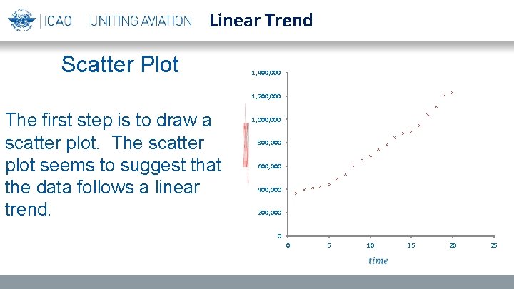
Linear Trend Scatter Plot 1, 400, 000 1, 200, 000 1, 000 800, 000 600, 000 400, 000 200, 000 0 The first step is to draw a scatter plot. The scatter plot seems to suggest that the data follows a linear trend. 0 5 10 15 20 25

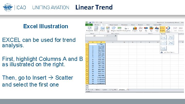
Linear Trend Excel Illustration EXCEL can be used for trend analysis. First, highlight Columns A and B as illustrated on the right. Then, go to Insert Scatter and select the first one

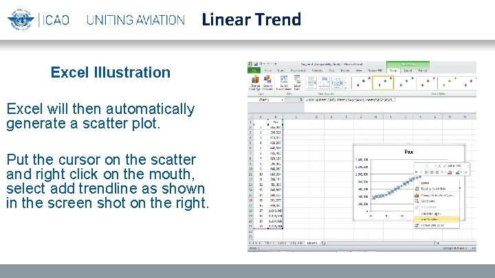
Linear Trend Excel Illustration Excel will then automatically generate a scatter plot. Put the cursor on the scatter and right click on the mouth, select add trendline as shown in the screen shot on the right.

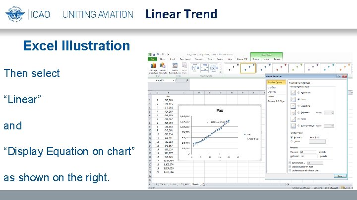
Linear Trend Excel Illustration Then select “Linear” and “Display Equation on chart” as shown on the right.

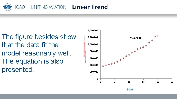
Linear Trend 1, 400, 000 The figure besides show that the data fit the model reasonably well. The equation is also presented. 1, 200, 000 R 2 = 0. 9809 1, 000 800, 000 600, 000 400, 000 200, 000 0 0 5 10 15 20 25

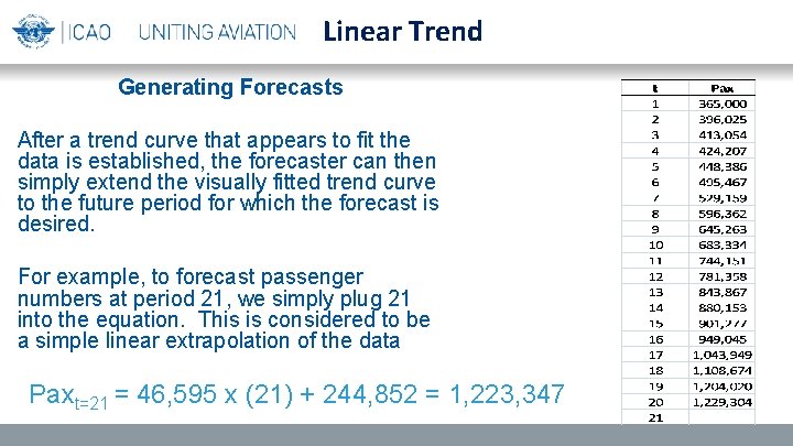
Linear Trend Generating Forecasts After a trend curve that appears to fit the data is established, the forecaster can then simply extend the visually fitted trend curve to the future period for which the forecast is desired. For example, to forecast passenger numbers at period 21, we simply plug 21 into the equation. This is considered to be a simple linear extrapolation of the data Paxt=21 = 46, 595 x (21) + 244, 852 = 1, 223, 347

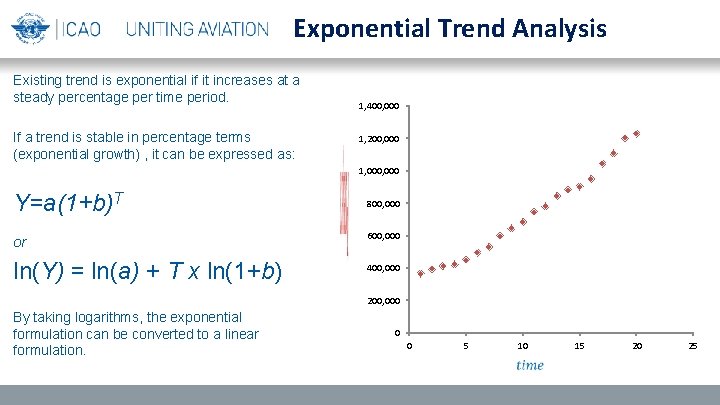
Exponential Trend Analysis Existing trend is exponential if it increases at a steady percentage per time period. 1, 400, 000 If a trend is stable in percentage terms (exponential growth) , it can be expressed as: 1, 200, 000 1, 000 Y=a(1+b)T 800, 000 or 600, 000 ln(Y) = ln(a) + T x ln(1+b) 400, 000 By taking logarithms, the exponential formulation can be converted to a linear formulation. 200, 000 0 0 5 10 15 20 25

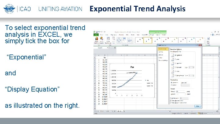
Exponential Trend Analysis To select exponential trend analysis in EXCEL, we simply tick the box for “Exponential” and “Display Equation” as illustrated on the right.

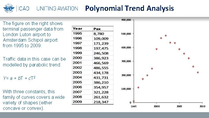
Polynomial Trend Analysis The figure on the right shows terminal passenger data from London Luton airport to Amsterdam Schipol airport from 1995 to 2009. Traffic data in this case can be modelled by parabolic trend: Y= a + b. T + c. T 2 With three constants, this family of curves covers a wide variety of shapes (either concave or convex). 600, 000 500, 000 400, 000 300, 000 200, 000 100, 000 0 1995 2000 2005 2010

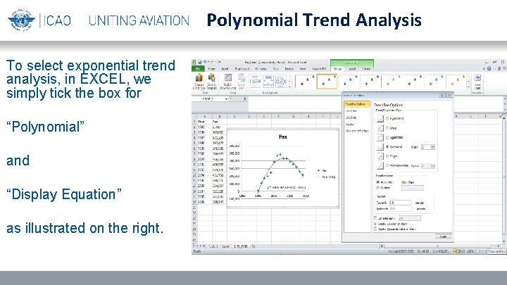
Polynomial Trend Analysis To select exponential trend analysis, in EXCEL, we simply tick the box for “Polynomial” and “Display Equation” as illustrated on the right.

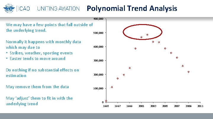
Polynomial Trend Analysis 600, 000 We may have a few points that fall outside of the underlying trend. 500, 000 Normally it happens with monthly data which may due to • Strikes, weather, sporting events • Easter tends to move around Do nothing if no substantial effects on estimation May remove them from the data May ‘adjust’ them to fit in with the underlying trend 400, 000 300, 000 200, 000 100, 000 0 1995 1997 1999 2001 2003 2005 2007 2009 2011

Introduction to Regression Analysis

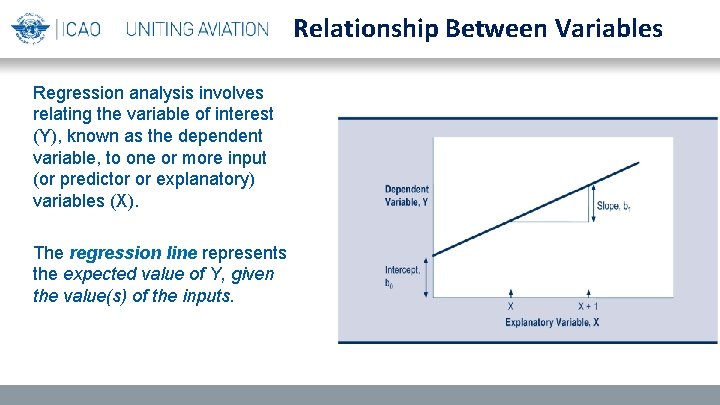
Relationship Between Variables Regression analysis involves relating the variable of interest (Y), known as the dependent variable, to one or more input (or predictor or explanatory) variables (X). The regression line represents the expected value of Y, given the value(s) of the inputs.

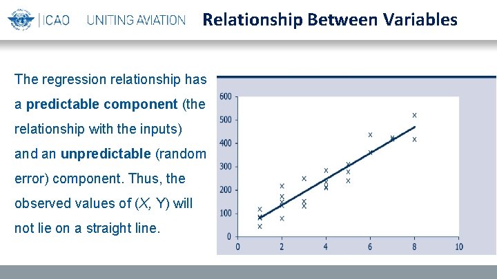
Relationship Between Variables The regression relationship has a predictable component (the relationship with the inputs) and an unpredictable (random error) component. Thus, the observed values of (X, Y) will not lie on a straight line.

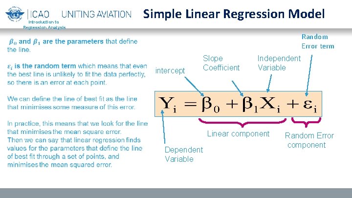
Introduction to Regression Analysis Simple Linear Regression Model Random Error term intercept Slope Coefficient Independent Variable Linear component Dependent Variable Random Error component

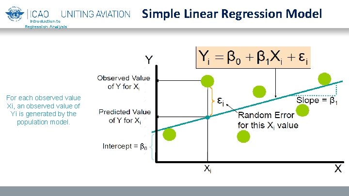
Introduction to Regression Analysis For each observed value Xi, an observed value of Yi is generated by the population model. Simple Linear Regression Model

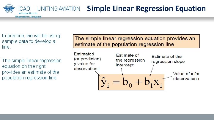
Introduction to Regression Analysis In practice, we will be using sample data to develop a line. The simple linear regression equation on the right provides an estimate of the population regression line. Simple Linear Regression Equation

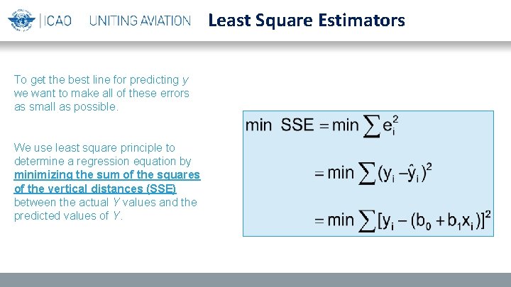
Least Square Estimators To get the best line for predicting y we want to make all of these errors as small as possible. We use least square principle to determine a regression equation by minimizing the sum of the squares of the vertical distances (SSE) between the actual Y values and the predicted values of Y.

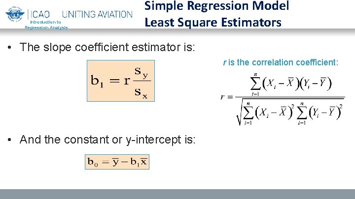
Introduction to Regression Analysis Simple Regression Model Least Square Estimators • The slope coefficient estimator is: r is the correlation coefficient: • And the constant or y-intercept is:

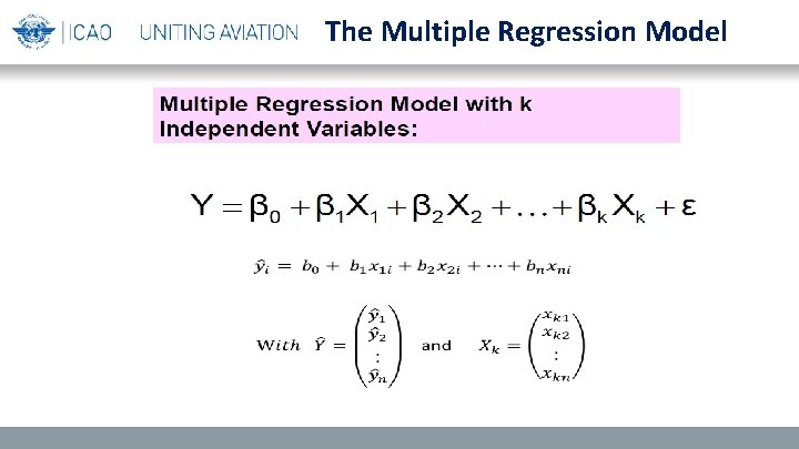
The Multiple Regression Model

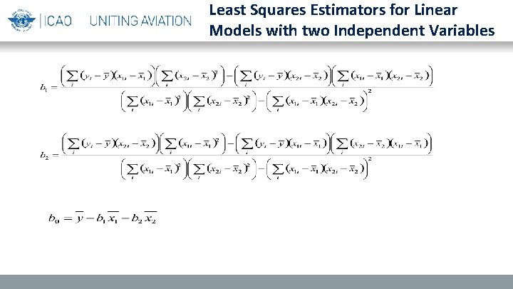
Least Squares Estimators for Linear Models with two Independent Variables

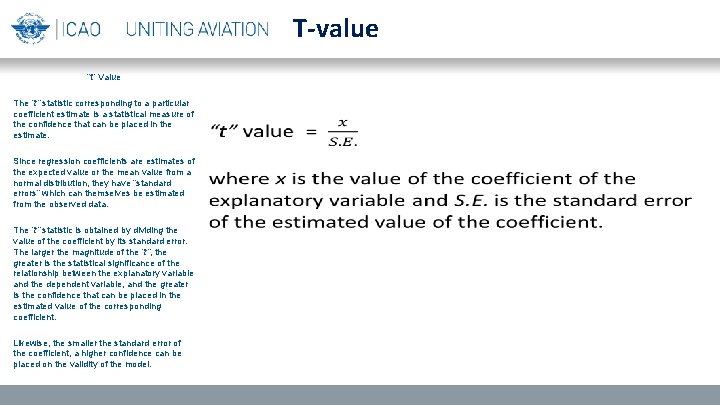
T-value “t” Value The “t” statistic corresponding to a particular coefficient estimate is a statistical measure of the confidence that can be placed in the estimate. Since regression coefficients are estimates of the expected value or the mean value from a normal distribution, they have “standard errors” which can themselves be estimated from the observed data. The “t” statistic is obtained by dividing the value of the coefficient by its standard error. The larger the magnitude of the “t”, the greater is the statistical significance of the relationship between the explanatory variable and the dependent variable, and the greater is the confidence that can be placed in the estimated value of the corresponding coefficient. Likewise, the smaller the standard error of the coefficient, a higher confidence can be placed on the validity of the model.

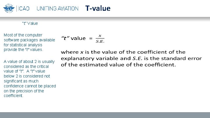
T-value “t” Value Most of the computer software packages available for statistical analysis provide the “t” values. A value of about 2 is usually considered as the critical value of “t”. A “t” value below 2 is considered not significant as much confidence cannot be placed on the precision of the coefficient.

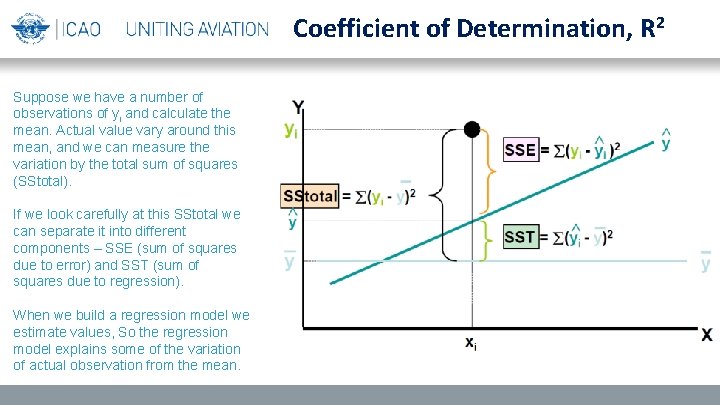
Coefficient of Determination, R 2 Suppose we have a number of observations of yi and calculate the mean. Actual value vary around this mean, and we can measure the variation by the total sum of squares (SStotal). If we look carefully at this SStotal we can separate it into different components – SSE (sum of squares due to error) and SST (sum of squares due to regression). When we build a regression model we estimate values, So the regression model explains some of the variation of actual observation from the mean.

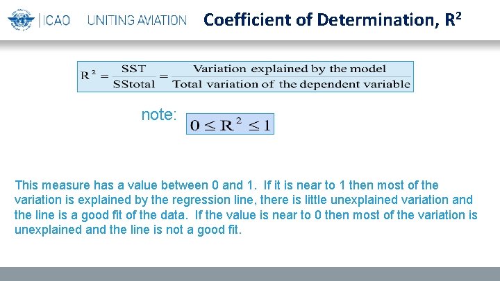
Coefficient of Determination, R 2 note: This measure has a value between 0 and 1. If it is near to 1 then most of the variation is explained by the regression line, there is little unexplained variation and the line is a good fit of the data. If the value is near to 0 then most of the variation is unexplained and the line is not a good fit.

Multiple Linear Regression Least Square Estimators We have to calculate the coefficients for each of the independent variable, but after seeing the arithmetic for multiple regression with two independent variables in the previous slide, you might guess, quite rightly, that the arithmetic is even more messy for a regression with more than two independent variables. This is why multiple regression is never tackled by hand. Thankfully, a lot of standard software includes multiple regression as a standard function. Too complicated by hand!

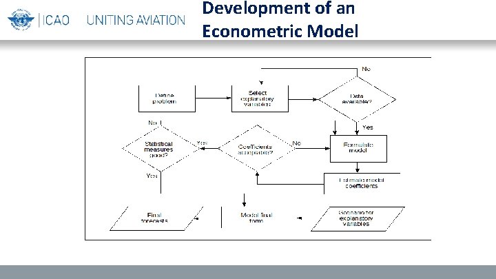
Development of an Econometric Model

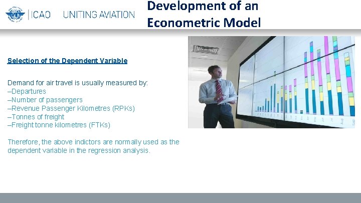
Development of an Econometric Model Selection of the Dependent Variable Demand for air travel is usually measured by: –Departures –Number of passengers –Revenue Passenger Kilometres (RPKs) –Tonnes of freight –Freight tonne kilometres (FTKs) Therefore, the above indictors are normally used as the dependent variable in the regression analysis.

Development of an Econometric Model Polynomial Trend Analysis Selection of Explanatory Variables The explanatory variables are expected to represent an important influence on demand in the particular circumstances. The explanatory variables should be chosen from those that are available from reliable sources. The explanatory variables should be independently predicted, either by a reliable independent source or by the forecaster

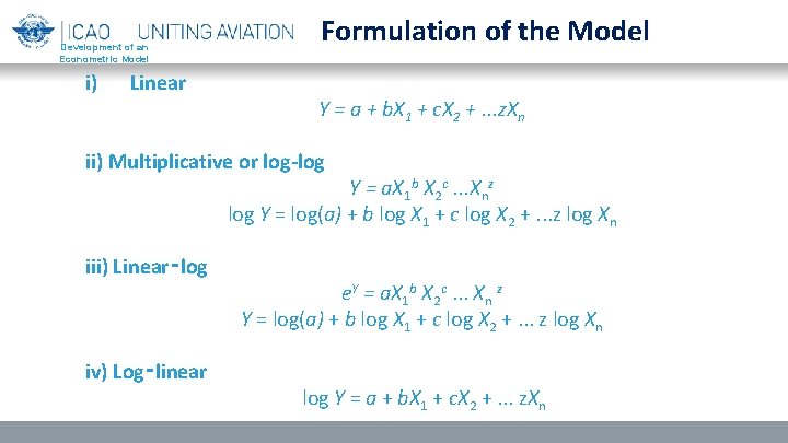
Development of an Econometric Model i) Linear Formulation of the Model Y = a + b. X 1 + c. X 2 +. . . z. Xn ii) Multiplicative or log-log Y = a. X 1 b X 2 c. . . Xnz log Y = log(a) + b log X 1 + c log X 2 +. . . z log Xn iii) Linear‑log iv) Log‑linear e. Y = a. X 1 b X 2 c. . . Xn z Y = log(a) + b log X 1 + c log X 2 +. . . z log Xn log Y = a + b. X 1 + c. X 2 +. . . z. Xn