IB 372 Lab 1 Introduction to Statistics Fall

IB 372 Lab 1: Introduction to Statistics Fall 2010

Thanks to Steve Paton - Smithsonian Tropical Research Institute for providing original spanish version of this file…

What are statistics? • Statistics are numbers used to: Describe and draw conclusions about DATA • These are called descriptive (or “univariate”) and inferential (or “analytical”) statistics, respectively.
Statistic vs. Parameter Formally (and somewhat confusingly): • A statistic is a measure of some attribute of a sample. • Whereas, a parameter is the real and unique measure of the attribute for the whole population. • Usually, the population is too big to measure, so in practice, statistics represent parameters. (thus, even “descriptive” stats are usually inferential too)
Variables • A variable is anything we can measure/observe • Three types: – Continuous: values span an uninterrupted range (e. g. height) – Discrete: only certain fixed values are possible (e. g. counts) – Categorical: values are qualitatively assigned (e. g. low/med/hi) • Dependence in variables: “Dependent variables depend on independent ones” – Independent variable may or may not be prescribed experimentally – Determining dependence is often not trivial!
Descriptive Statistics
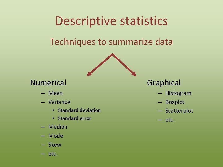
Descriptive statistics Techniques to summarize data Numerical – Mean – Variance • Standard deviation • Standard error – – Median Mode Skew etc. Graphical – – Histogram Boxplot Scatterplot etc.
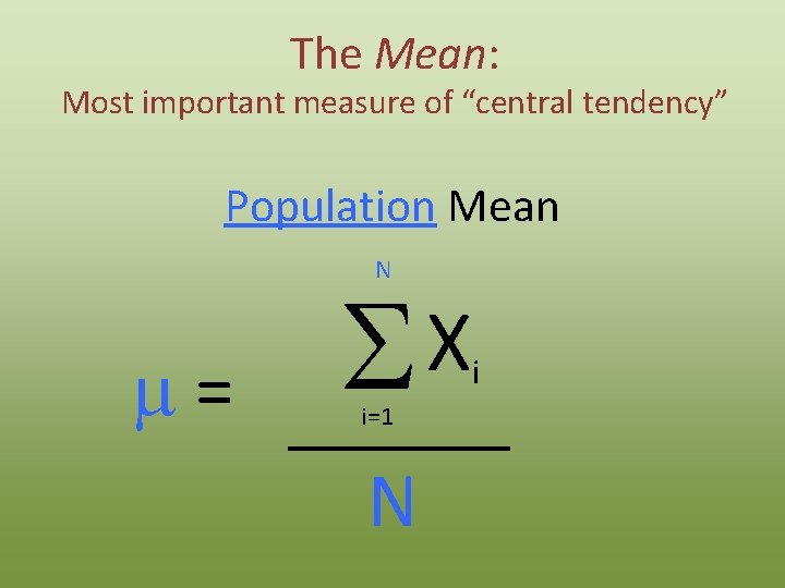
The Mean: Most important measure of “central tendency” Population Mean N m= X S i=1 N i
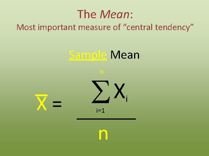
The Mean: Most important measure of “central tendency” Sample Mean n X= X S i=1 n i
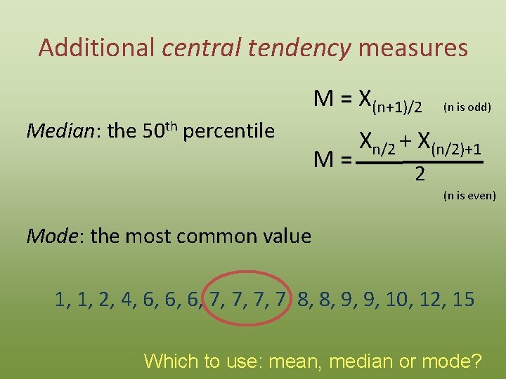
Additional central tendency measures Median: the 50 th percentile M = X(n+1)/2 M= (n is odd) Xn/2 + X(n/2)+1 2 (n is even) Mode: the most common value 1, 1, 2, 4, 6, 6, 6, 7, 7, 8, 8, 9, 9, 10, 12, 15 Which to use: mean, median or mode?
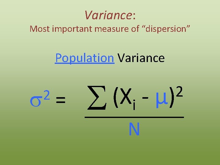
Variance: Most important measure of “dispersion” Population Variance 2 s = (X S i N 2 µ)
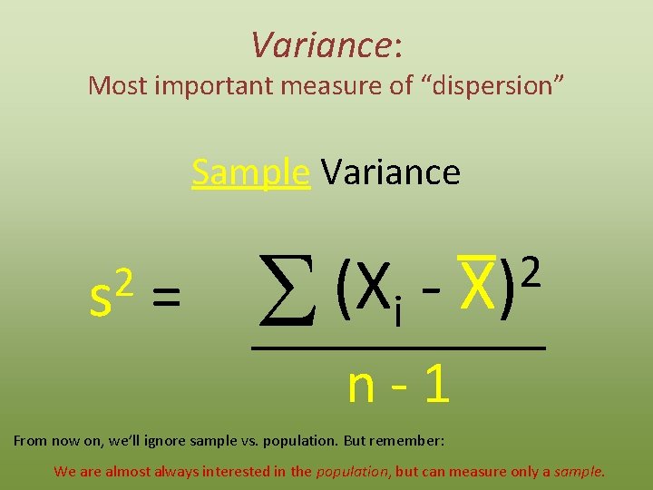
Variance: Most important measure of “dispersion” Sample Variance 2 s = (X S i 2 X) n-1 From now on, we’ll ignore sample vs. population. But remember: We are almost always interested in the population, but can measure only a sample.
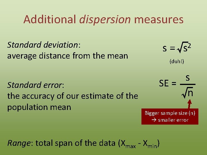
Additional dispersion measures Standard deviation: average distance from the mean Standard error: the accuracy of our estimate of the population mean s =√ s 2 (duh!) s SE = √n Bigger sample size (n) smaller error Range: total span of the data (Xmax - Xmin)
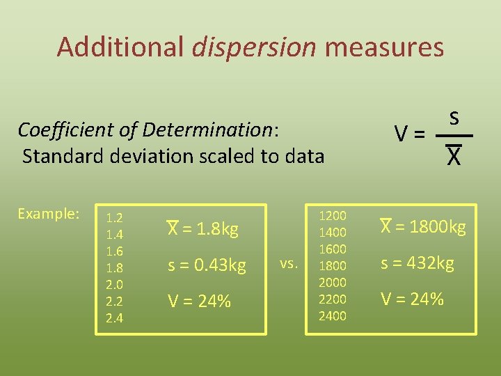
Additional dispersion measures Coefficient of Determination: Standard deviation scaled to data Example: 1. 2 1. 4 1. 6 1. 8 2. 0 2. 2 2. 4 X = 1. 8 kg s = 0. 43 kg V = 24% vs. 1200 1400 1600 1800 2000 2200 2400 s V= X X = 1800 kg s = 432 kg V = 24%

“Graphical Statistics”
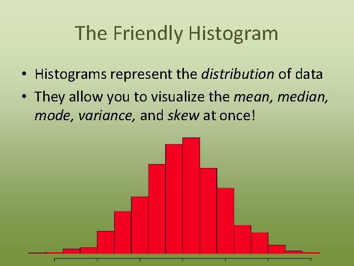
The Friendly Histogram • Histograms represent the distribution of data • They allow you to visualize the mean, median, mode, variance, and skew at once!
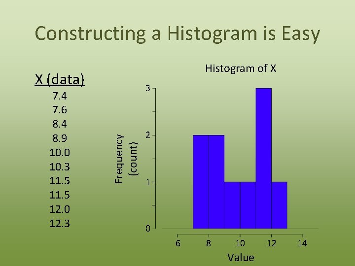
Constructing a Histogram is Easy Histogram of X X (data) Frequency (count) 7. 4 7. 6 8. 4 8. 9 10. 0 10. 3 11. 5 12. 0 12. 3 3 2 1 0 6 8 10 Value 12 14
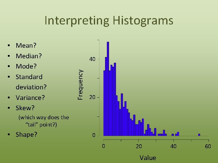
Interpreting Histograms 40 Frequency Mean? Median? Mode? Standard deviation? • Variance? • Skew? • • 20 (which way does the “tail” point? ) • Shape? 0 0 20 Value 40 60
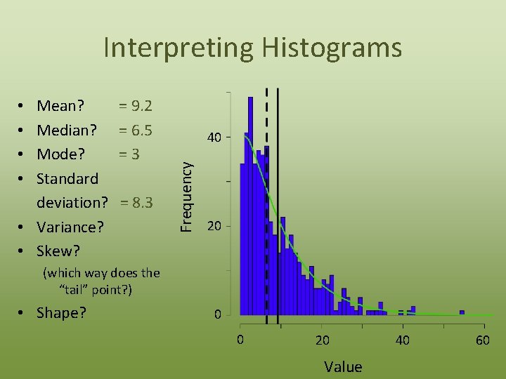
Interpreting Histograms = 9. 2 = 6. 5 =3 = 8. 3 40 Frequency Mean? Median? Mode? Standard deviation? • Variance? • Skew? • • 20 (which way does the “tail” point? ) • Shape? 0 0 20 Value 40 60
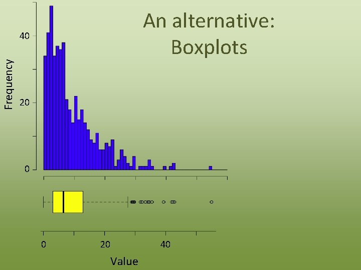
An alternative: Boxplots Frequency 40 20 0 0 20 40 Value
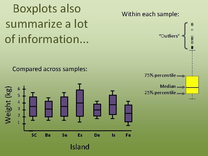
Boxplots also summarize a lot of information. . . Within each sample: “Outliers” Weight (kg) Compared across samples: 75% percentile Median 25% percentile 6 5 4 3 2 1 SC Ba Se Es Island Da Is Fe

Normality
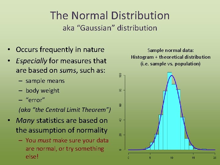
The Normal Distribution aka “Gaussian” distribution • Occurs frequently in nature • Especially for measures that are based on sums, such as: – sample means – body weight – “error” (aka “the Central Limit Theorem”) • Many statistics are based on the assumption of normality – You must make sure your data are normal, or try something else! Sample normal data: Histogram + theoretical distribution (i. e. sample vs. population)
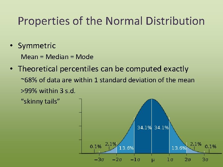
Properties of the Normal Distribution • Symmetric Mean = Median = Mode • Theoretical percentiles can be computed exactly ~68% of data are within 1 standard deviation of the mean >99% within 3 s. d. “skinny tails”
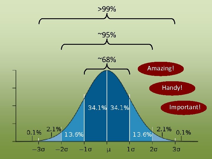
>99% ~95% ~68% Amazing! Handy! Important!
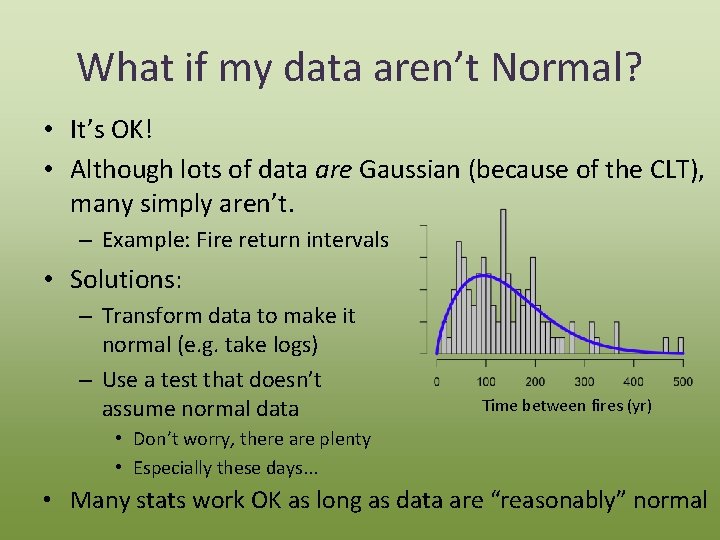
What if my data aren’t Normal? • It’s OK! • Although lots of data are Gaussian (because of the CLT), many simply aren’t. – Example: Fire return intervals • Solutions: – Transform data to make it normal (e. g. take logs) – Use a test that doesn’t assume normal data Time between fires (yr) • Don’t worry, there are plenty • Especially these days. . . • Many stats work OK as long as data are “reasonably” normal

Break!
Inferential Statistics: Introduction
Inference: the process by which we draw conclusions about an unknown based on evidence or prior experience. In statistics: make conclusions about a population based on samples taken from that population. Important: Your sample must reflect the population you’re interested in, otherwise your conclusions will be misleading!
Statistical Hypotheses • Should be related to a scientific hypothesis! • Very often presented in pairs: – Null Hypothesis (H 0): Usually the “boring” hypothesis of “no difference” – Alternative Hypothesis (HA) Usually the interesting hypothesis of “there is an effect” • Statistical tests attempt to (mathematically) reject the null hypothesis
Significance • Your sample will never match H 0 perfectly, even when H 0 is in fact true • The question is whether your sample is different enough from the expectation under H 0 to be considered significant • If your test finds a significant difference, then you reject H 0.
p-Values Measure Significance The p-value of a test is the probability of observing data at least as extreme as your sample, assuming H 0 is true • If p is very small, it is unlikely that H 0 is true (in other words, if H 0 were true, your observed sample would be unlikely) • How small does p have to be? – It’s up to you (depends on question) – 0. 05 is a common cutoff • If p<0. 05, then there is less than 5% chance that you would observe your sample if the null hypothesis was true.
‘Proof’ in statistics • Failing to reject (i. e. “accepting”) H 0 does not prove that H 0 is true! • And accepting HA doesn’t prove that HA is true either! Why? • Statistical inference tries to draw conclusions about the population from a small sample – By chance, the samples may be misleading – Example: if you always accept H 0 at p=0. 05, then 1 in 20 times you will be wrong!
Errors in Hypothesis Testing • Type I Error: Reject H 0 when H 0 is actually true – i. e. You find a difference when really there is none – The probability of Type I error is called the “significance level” of a test, and denoted α • Type II Error: Accept H 0 when H 0 is actually false – i. e. There really is a difference, but you conclude there is none – The probability of Type II error is denoted β (and [1 – β is called the “power” of the test)
Assumptions of inferential statistics • All inferential tests are based on assumptions – If your data cannot meet the assumptions, the test results are invalid! • In particular: – Inferential tests assume random sampling – Many tests assume the data fit a theoretical distribution (often normal) • These are “parametric tests” • Luckily, there are non-parametric alternatives
Inferential Statistics: Methods

Student’s t-Test
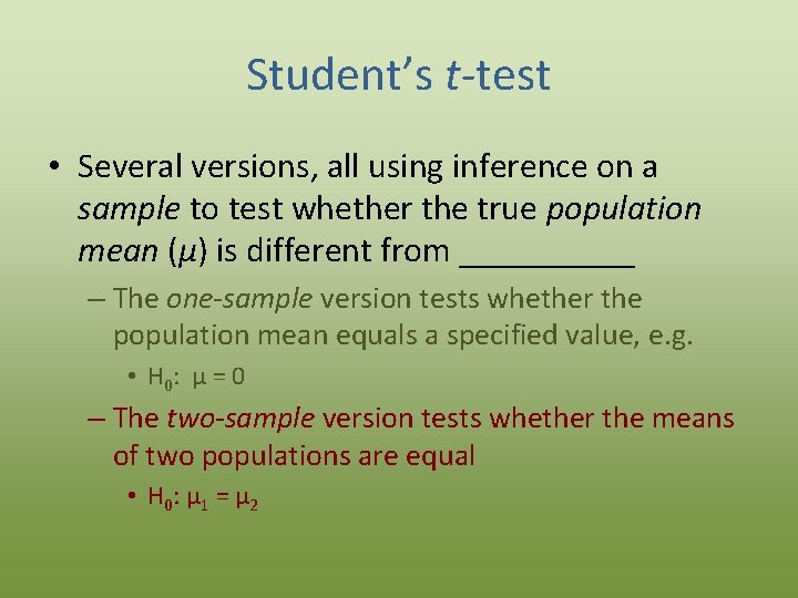
Student’s t-test • Several versions, all using inference on a sample to test whether the true population mean (µ) is different from _____ – The one-sample version tests whether the population mean equals a specified value, e. g. • H 0 : µ = 0 – The two-sample version tests whether the means of two populations are equal • H 0 : µ 1 = µ 2
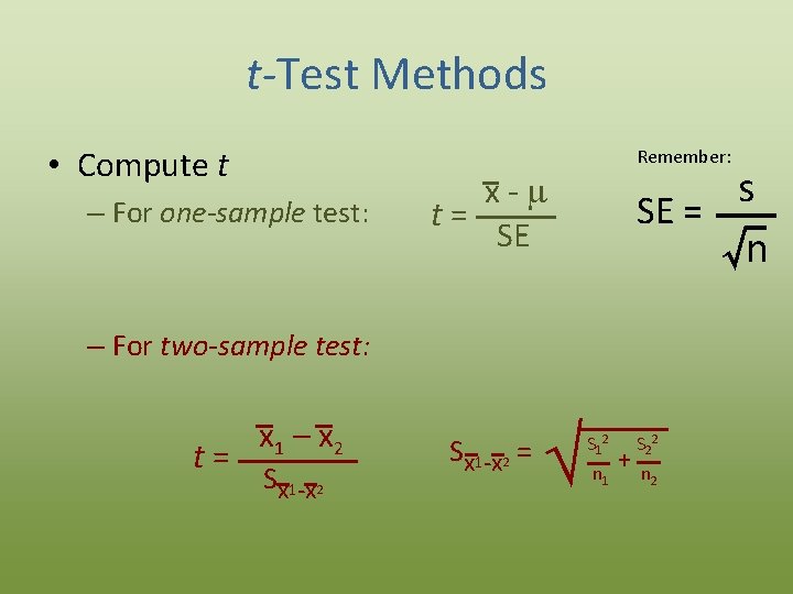
t-Test Methods • Compute t – For one-sample test: Remember: s SE = √n x-m t= SE – For two-sample test: t= x 1 – x 2 Sx 1 -x 2 = Ö S 12 n 1 + S 22 n 2
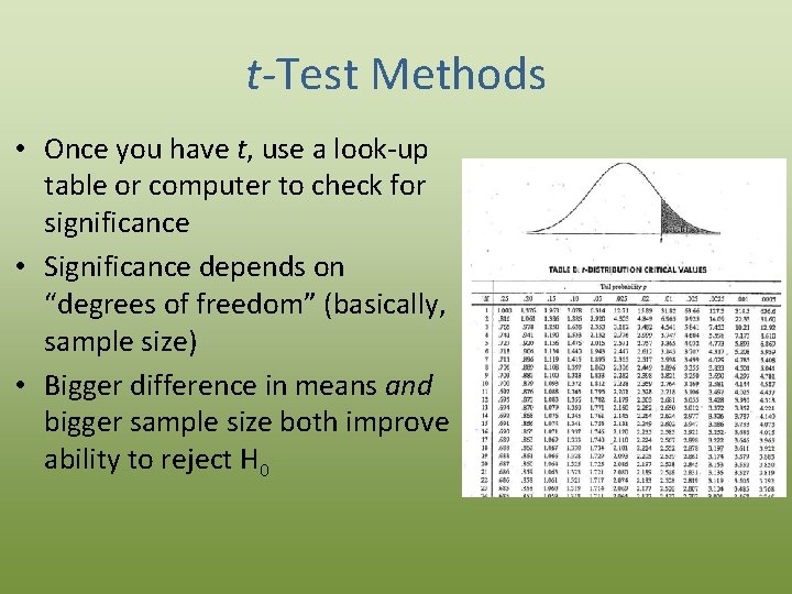
t-Test Methods • Once you have t, use a look-up table or computer to check for significance • Significance depends on “degrees of freedom” (basically, sample size) • Bigger difference in means and bigger sample size both improve ability to reject H 0
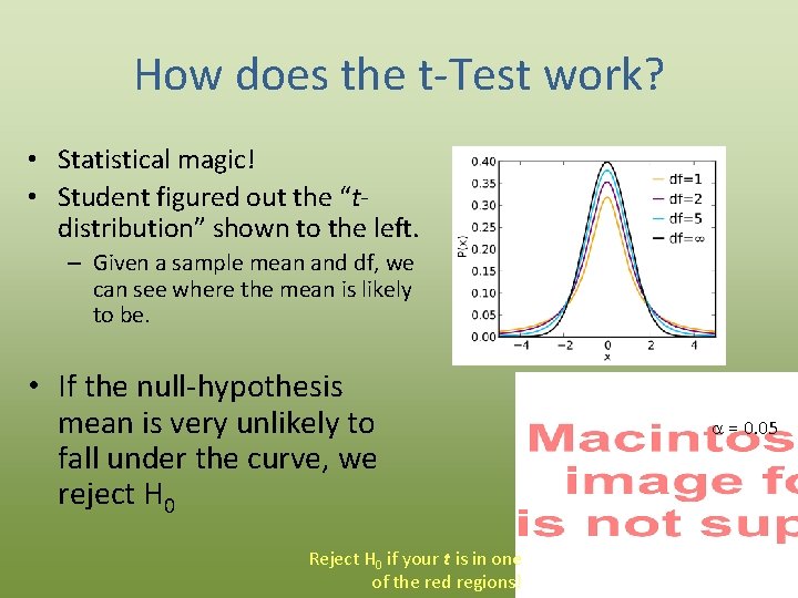
How does the t-Test work? • Statistical magic! • Student figured out the “tdistribution” shown to the left. – Given a sample mean and df, we can see where the mean is likely to be. • If the null-hypothesis mean is very unlikely to fall under the curve, we reject H 0 Reject H 0 if your t is in one of the red regions! a = 0. 05

Try it! Work through the Excel exercises for one- and two-sample t-tests now

ANOVA
ANOVA: ANalysis Of VAriance • Tests for significant effect of 1 or more factors • Each factor may have 2 or more levels • Can also test for interactions between factors • For just 1 factor with 2 levels, ANOVA = t-test – So why can’t we just do lots of t-tests for more complicated experiments? • Example: We study tree growth rates on clay vs. sand vs. loam soil (10 trees each) – How many factors? How many levels for each factor?
ANOVA: Concept • Despite the name, ANOVA really looks for difference in means between groups (factors & levels) • To do so, we partition the variability in our data into: – (1) The variability that can be explained by factors – (2) The leftover unexplained variability (error or residual variability) Total variability = Variability due to factors + error (we only have to calculate two of these values)
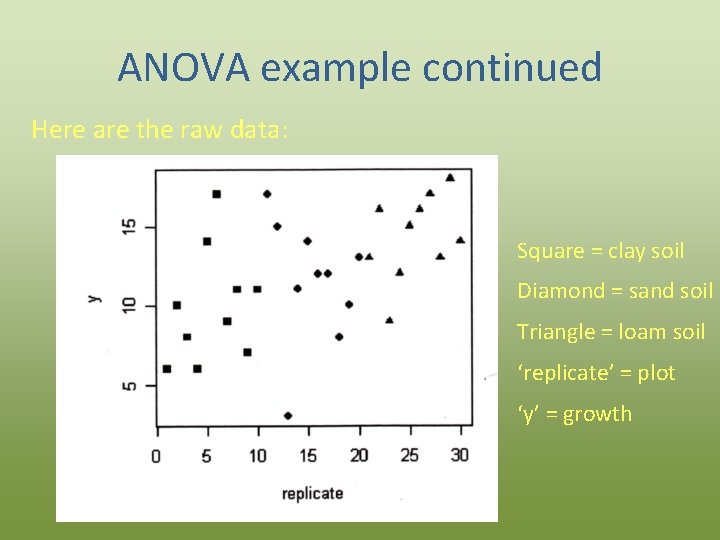
ANOVA example continued Here are the raw data: Square = clay soil Diamond = sand soil Triangle = loam soil ‘replicate’ = plot ‘y’ = growth
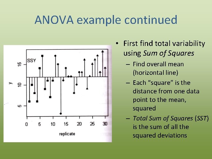
ANOVA example continued • First find total variability using Sum of Squares – Find overall mean (horizontal line) – Each “square” is the distance from one data point to the mean, squared – Total Sum of Squares (SST) is the sum of all the squared deviations
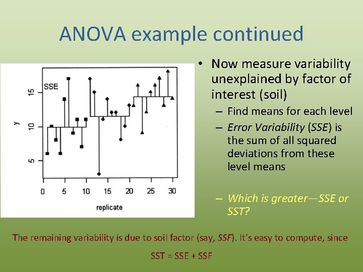
ANOVA example continued • Now measure variability unexplained by factor of interest (soil) – Find means for each level – Error Variability (SSE) is the sum of all squared deviations from these level means – Which is greater—SSE or SST? The remaining variability is due to soil factor (say, SSF). It’s easy to compute, since SST = SSE + SSF
ANOVA example continued • Next, we calculate degrees of freedom (df ) – df is based mainly on sample size – Every time you estimate a parameter from your data, you lose one df • Example: Since we computed the mean of our 30 observations, we only need to know 29 of the values now to determine the last one! • For our example we have: df. SST = 30 – 1 = 29 df. SSE = (10 – 1) + (10 – 1) = 27 df. SSF = df. SST – df. SSE = 2
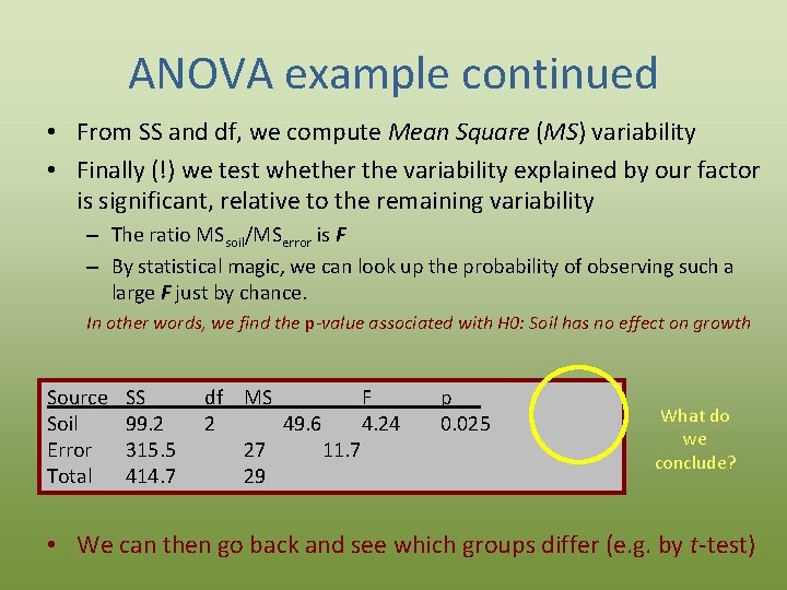
ANOVA example continued • From SS and df, we compute Mean Square (MS) variability • Finally (!) we test whether the variability explained by our factor is significant, relative to the remaining variability – The ratio MSsoil/MSerror is F – By statistical magic, we can look up the probability of observing such a large F just by chance. In other words, we find the p-value associated with H 0: Soil has no effect on growth Source Soil Error Total SS 99. 2 315. 5 414. 7 df MS F 2 49. 6 4. 24 27 11. 7 29 p 0. 025 What do we conclude? • We can then go back and see which groups differ (e. g. by t-test)

Try it! Work through the Excel exercise for ANOVA now
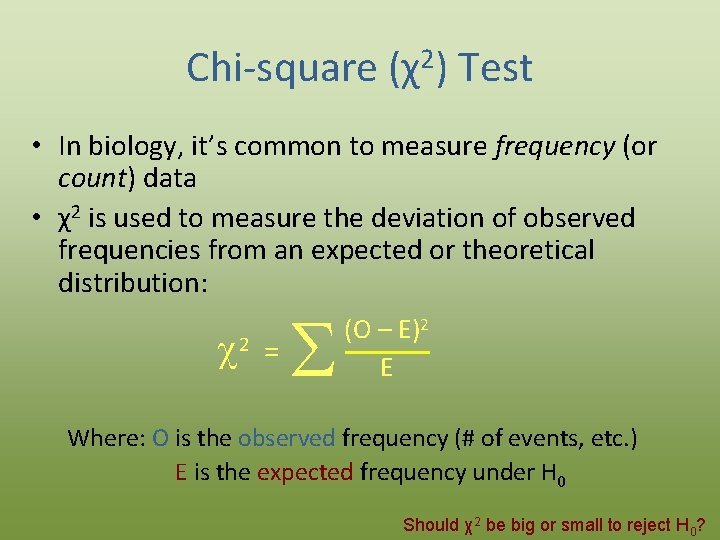
Chi-square (χ2) Test • In biology, it’s common to measure frequency (or count) data • χ2 is used to measure the deviation of observed frequencies from an expected or theoretical distribution: c 2 = S (O – E)2 E Where: O is the observed frequency (# of events, etc. ) E is the expected frequency under H 0 Should χ2 be big or small to reject H 0?
χ2 Example • Again we’ll also need to know degrees of freedom • For the χ2 test, df = number of groups – 1 • Then (again by statistical magic), we can look up how big χ2 needs to be (the critical value) to reject H 0 at a given significance level
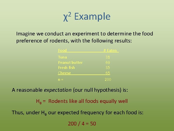
χ2 Example Imagine we conduct an experiment to determine the food preference of rodents, with the following results: Food # Eaten Tuna Peanut butter Fresh fish Cheese 31 69 35 65 n= 200 A reasonable expectation (our null hypothesis) is: H 0 = Rodents like all foods equally well Thus, under H 0 our expected frequency for each food is: 200 / 4 = 50
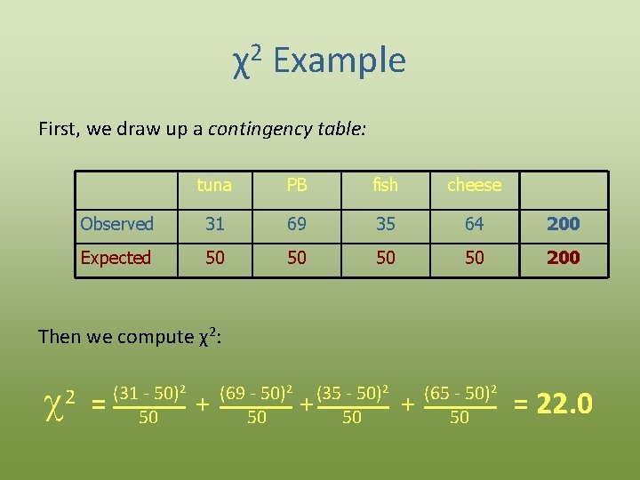
χ2 Example First, we draw up a contingency table: tuna PB fish cheese Observed 31 69 35 64 200 Expected 50 50 200 Then we compute χ2: c = 2 (31 - 50)2 50 + (69 - 50)2 50 (35 - 50)2 + 50 + (65 - 50)2 50 = 22. 0
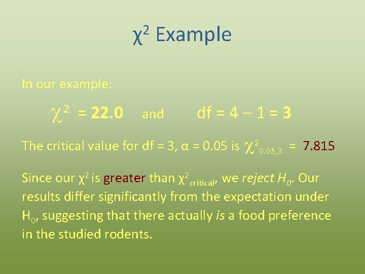
χ2 Example In our example: c 2 = 22. 0 and df = 4 – 1 = 3 The critical value for df = 3, α = 0. 05 is c 20. 05, 3 = 7. 815 Since our χ2 is greater than χ2 critical, we reject H 0. Our results differ significantly from the expectation under H 0, suggesting that there actually is a food preference in the studied rodents.

Try it! Work through the Excel exercise for the Chi-square test now
Correlation • Correlation measures the strength of the relationship between two variables – When X gets larger, does Y consistently get larger (or smaller)? • Often measured with Pearson’s correlation coefficient – Usually just called “correlation coefficient” – Almost always represented with the letter r
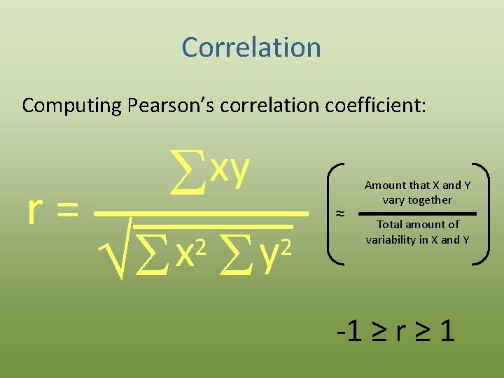
Correlation Computing Pearson’s correlation coefficient: r= xy S x ÖS 2 y S ≈ 2 Amount that X and Y vary together Total amount of variability in X and Y -1 ≥ r ≥ 1
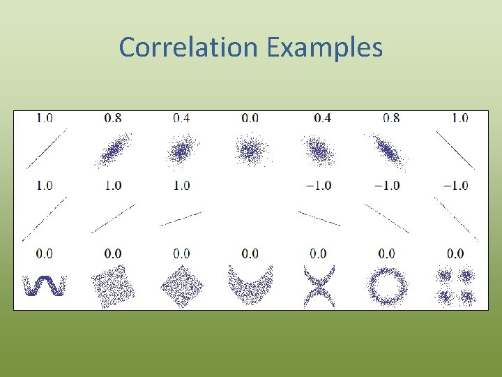
Correlation Examples
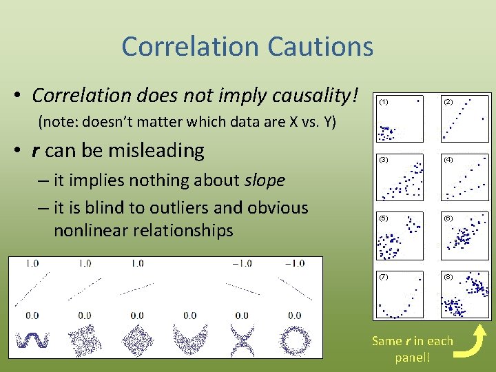
Correlation Cautions • Correlation does not imply causality! (note: doesn’t matter which data are X vs. Y) • r can be misleading – it implies nothing about slope – it is blind to outliers and obvious nonlinear relationships Same r in each panel!

Try it! Work through the Excel exercise for correlations now
Regression • Unlike correlation, regression does imply a functional relationship between variables – The dependent variable is a function of the independent variable(s) • In regression, you propose an algebraic model, then find the “best fit” to your data – Most commonly, the model is a simple line (“Y is a linear function of X”)
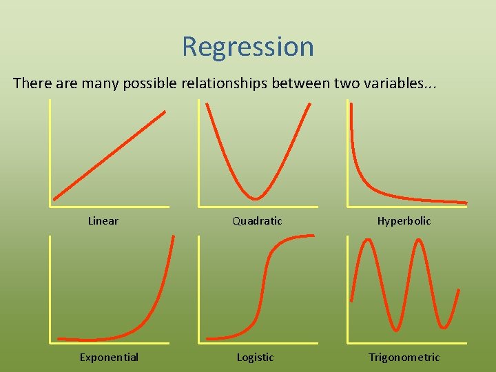
Regression There are many possible relationships between two variables. . . Linear Exponential Quadratic Hyperbolic Logistic Trigonometric
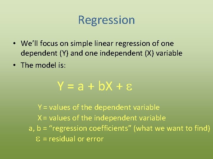
Regression • We’ll focus on simple linear regression of one dependent (Y) and one independent (X) variable • The model is: Y = a + b. X + Y = values of the dependent variable X = values of the independent variable a, b = “regression coefficients” (what we want to find) = residual or error
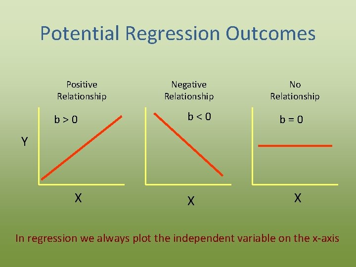
Potential Regression Outcomes Positive Relationship b>0 Negative Relationship b<0 No Relationship b=0 Y X X X In regression we always plot the independent variable on the x-axis
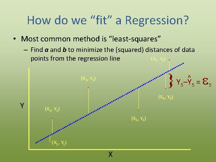
How do we “fit” a Regression? • Most common method is “least-squares” – Find a and b to minimize the (squared) distances of data (X 4, Y 4). points from the regression line Y –Y = . (X 3, Y 3) . Y 5 (X 5, Y 5) . (X 2, Y 2) . (X 6, Y 6) . (X 1, Y 1) X ^ 5 5
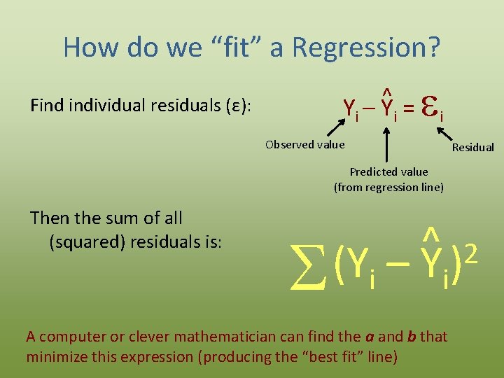
How do we “fit” a Regression? Find individual residuals (ε): ^ Yi – Y i = i Observed value Residual Predicted value (from regression line) Then the sum of all (squared) residuals is: (Y – S i ^ 2 Y i) A computer or clever mathematician can find the a and b that minimize this expression (producing the “best fit” line)
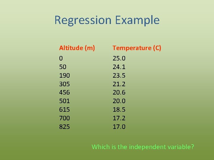
Regression Example Altitude (m) 0 50 190 305 456 501 615 700 825 Temperature (C) 25. 0 24. 1 23. 5 21. 2 20. 6 20. 0 18. 5 17. 2 17. 0 Which is the independent variable?
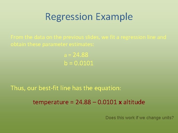
Regression Example From the data on the previous slides, we fit a regression line and obtain these parameter estimates: a = 24. 88 b = 0. 0101 Thus, our best-fit line has the equation: temperature = 24. 88 – 0. 0101 x altitude Does this work if we change units?
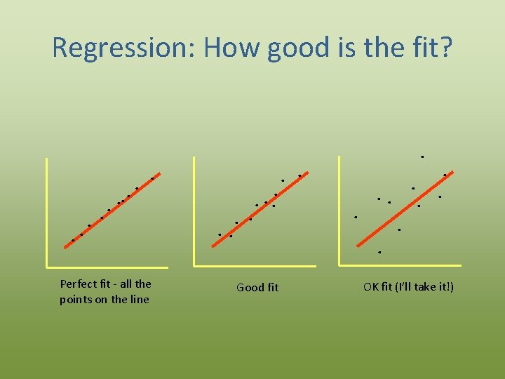
Regression: How good is the fit? . . Perfect fit - all the points on the line . . Good fit OK fit (I’ll take it!)
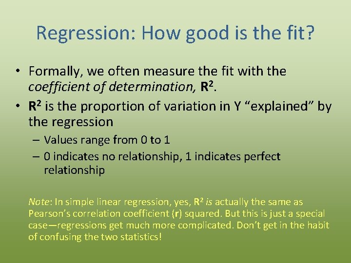
Regression: How good is the fit? • Formally, we often measure the fit with the coefficient of determination, R 2. • R 2 is the proportion of variation in Y “explained” by the regression – Values range from 0 to 1 – 0 indicates no relationship, 1 indicates perfect relationship Note: In simple linear regression, yes, R 2 is actually the same as Pearson’s correlation coefficient (r) squared. But this is just a special case—regressions get much more complicated. Don’t get in the habit of confusing the two statistics!
Regression: Is the fit significant? • We usually ask whether R 2 is significant by testing the null hypothesis: H 0: b = 0 (the line may as well be flat) against the alternative: HA: b ≠ 0 (the best fit isn’t a flat line) • Luckily (statistical magic), this can be tested with the t-test! – Depends on degrees of freedom (increase sample size to improve significance) – For our purposes, statistics software will do this for you
Regression Reservations • Again, regression does imply causality (unlike correlation), but importantly, it still does not test a causal biological relationship – Some other variable might affect both X and Y – You could even have the relationship backwards! • Be careful extrapolating regression lines: – beyond the original data range, or – to other populations
Try it! Work through the Excel exercise for simple linear regression now
- Slides: 75