Hypothesis Testing Slides by Deborah Nolan deborahnolanberkeley edu

Hypothesis Testing Slides by: Deborah Nolan deborah_nolan@berkeley. edu Sp 18 updates: Fernando Perez fernando. perez@Berkeley. edu ?

Examples Ø Excess Deaths on a Nurse’s Shifts Ø Introduction to Concepts in a Hypothesis Test Ø Student Evaluation of Teaching Ø Permutation tests

1. United States v. Kristen Gilbert (from Cobb and Gehlbach, “Statistics in the Courtroom”, in Statistics: A Guide to the Unknown)

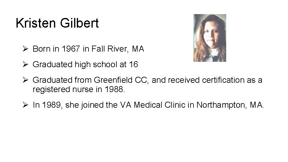
Kristen Gilbert Ø Born in 1967 in Fall River, MA Ø Graduated high school at 16 Ø Graduated from Greenfield CC, and received certification as a registered nurse in 1988. Ø In 1989, she joined the VA Medical Clinic in Northampton, MA.

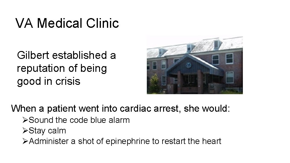
VA Medical Clinic Gilbert established a reputation of being good in crisis When a patient went into cardiac arrest, she would: ØSound the code blue alarm ØStay calm ØAdminister a shot of epinephrine to restart the heart

Suspicions Ø By the mid 1990’s, other nurses had become suspicious of Gilbert. Ø It seemed there were too many code blue calls, too many crises when Gilbert was on the ward. Ø An initial VA report found that the number of deaths were consistent with patterns at other VA hospitals. Ø The suspicions of the staff remained.

Suspicions Ø The staff brought their concerns again to the administration of the VAMC. Ø They hired a statistician as a consultant to look into the situation (Gehlbach) Ø His findings agreed with the staff concerns.

Assistant U. S. Attorney Welch convened a grand jury in 1998 to hear the evidence against Gilbert.

Grand Jury Ø A grand jury determines whethere is enough evidence for a trial. Ø The grand jury examines evidence and issues an indictment or not. The indictment is a formal accusation that a person has committed a crime.

Evidence Considered for Indictment Ø Motivation – Gilbert liked the thrill of a crisis, needed the recognition, and wanted to impress her boyfriend who also worked at the VAMC. Ø Testimony of co-workers about access Gilbert had to epinephrine. Ø Testimony of a physician about the symptoms of the men (healthy, middle-aged, not typical candidates for cardiac arrest).

Convincing? Ø No one had seen Gilbert give fatal injections. Ø A major part of the evidence for indictment was statistical.

QUESTION Were there so many excess deaths when Gilbert was present as to be suspicious in the eyes of science?

Gelbach’s Testimony 1. EDA and Visualization - Pattern of deaths, by shift and by year on the medical ward where Gilbert worked 2. Simulation - Variability in a chance process 3. Hypothesis Test – Was the pattern of excess deaths on Gilbert’s shifts too extreme to be regarded as ordinary, expected variability

Pattern of Deaths Ø The plot shows data from the VAMC. Ø Each point represents one year’s worth of data for a particular shift (night, day, evening). Ø The red points are those years (and shifts) that Gilbert worked at the VA. Gilbert started on the night shift in Mar ‘ 90, and left in Feb ‘ 96 Ø Look at the pattern from one year to the next.

Pattern of Deaths

Pattern in Deaths Ø There is a clear pattern associating Gilbert’s presence with excess deaths Ø However, the pattern might be nothing more than the result of ordinary, expectable variation.

Assess the Variation Ø Consider the 18 months leading up to Feb 1996, when Gilbert went on medical leave. Ø There were 547 days in this 18 month period and 3 shifts a day, for a total of 1641 shifts Ø For each shift, we have whether or not Gilbert worked the shift and whether or not there was a death on the shift.

Data – Two 0 -1 indicator variables Ø 1641 records Ø Was Gilbert working? 0 = No, 1 = Yes Ø Was there a death on the shift? 0 = No, 1 = Yes Ø What is the joint distribution of these two indicators?

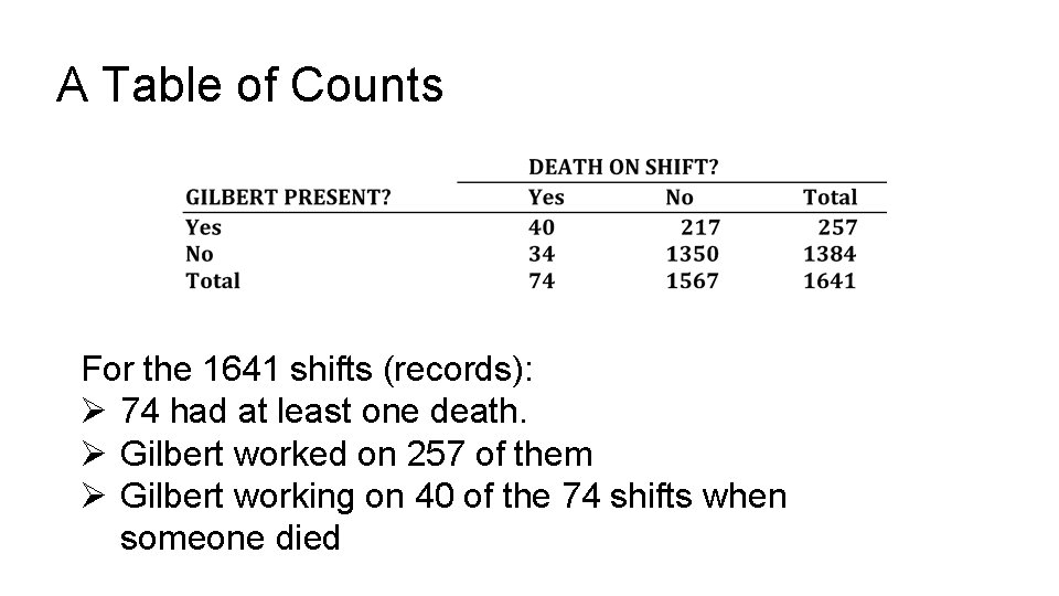
A Table of Counts For the 1641 shifts (records): Ø 74 had at least one death. Ø Gilbert worked on 257 of them Ø Gilbert working on 40 of the 74 shifts when someone died

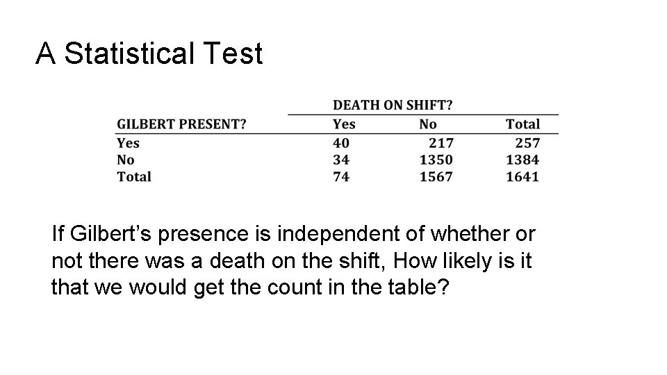
A Statistical Test If Gilbert’s presence is independent of whether or not there was a death on the shift, How likely is it that we would get the count in the table?

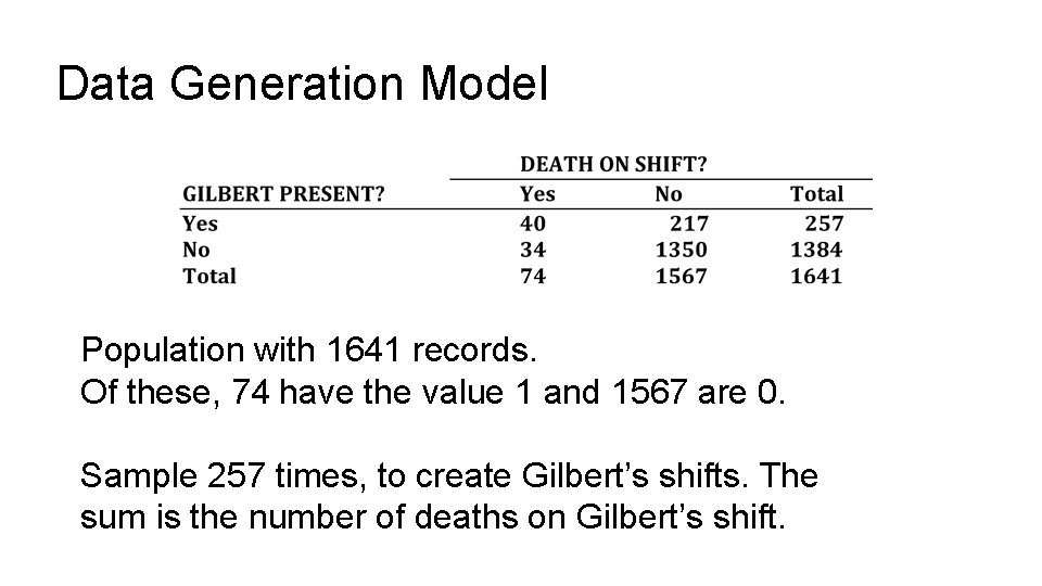
Data Generation Model Population with 1641 records. Of these, 74 have the value 1 and 1567 are 0. Sample 257 times, to create Gilbert’s shifts. The sum is the number of deaths on Gilbert’s shift.

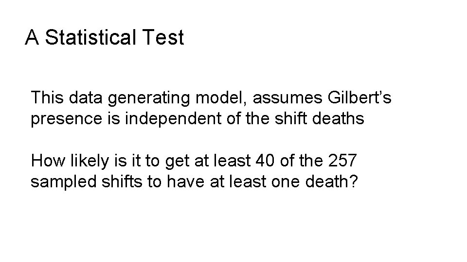
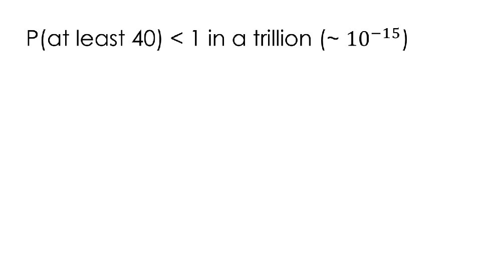
A Statistical Test This data generating model, assumes Gilbert’s presence is independent of the shift deaths How likely is it to get at least 40 of the 257 sampled shifts to have at least one death?

Hypothesis Test Ø Assume Gilbert’s presence and death on a shift are independent Ø Under this model for generating the data, what is the chance we would see an outcome as extreme as the one that we saw? Ø The chance is so rare that we reject the model of independence.

T/F Statements http: //bit. ly/ds 100 -sp 18 -? ? ? Ø The chance is less than 1 in a billion that Gilbert is innocent. Ø Gilbert was not assigned to her shifts at random so this probability calculation is flawed Ø The probability is so small that we’re sure Gilbert’s shifts are not independent of whether or not there was a death, but that doesn’t prove she’s guilty. There could be other explanations.

Grand Jury Ø The grand jury found the statistical evidence persuasive Ø Gilbert was indicted Ø The VA hospital is legal property of the federal government so it was a federal indictment. Ø Trial would be in federal district court, and the death penalty would be a possible sentence, if found guilty.

The Trial Ø The petit jury (or trial jury) hears the evidence in a trial as presented by both the plaintiff and the defendant. Ø After hearing the evidence, the group retires for deliberation, to consider a verdict. Ø The majority required for a guilty verdict was a simple majority (7 put of 12). A unanimous verdict for the sentence was needed for the death penalty.

Expert Witness Ø The court system allows expert testimony when the evidence involves specialized technical or scientific issues that go beyond what jurors would ordinarily be familiar with. Ø The experts help the jury understand the evidence better. Ø Supreme Court has set guidelines to make sure unscientific testimony is not admitted. Ø If there is expert testimony on one side, attorneys for the other side sometimes hire another expert who will disagree and “cancel out” the other expert.

QUESTION: Should the trial jury be allowed to hear the statistical evidence?

Report to the Judge Ø Was the statistical analysis done correctly? Ø What does the probability calculation NOT tell you? Ø Association vs Causation: Conclusions drawn from an Observational Study vs a Designed Experiment Ø Prosecutor’s Fallacy: Probability computed under assumptions of innocence

Was the statistical analysis done correctly? Ø The Defense Statistician (Cobb) agreed with the analysis performed by the Prosecution Statistician for the grand jury. Ø The excess deaths was an extremely unlikely outcome due to chance variation. Ø The pattern of deaths justified the indictment. Ø No need to bring statistical evidence to trial.

Association vs Causation Ø In a well-designed experiment, e. g. the clinical trials, where the subjects have been assigned at random to difference treated and control groups, the two groups resemble each other in most all ways, except for the receipt of the treatment. Ø The tiny probability rules out chance variation, and the conclusion is that the difference is “real”. Ø In this case, we can conclude that the explanation for the observed difference is the treatment.

Association vs Causation Ø The Gilbert case was NOT a randomized controlled experiment. (Gilbert’s presence on the ward would have had to be assigned using a chance device). Ø We can conclude that the difference is not due to chance variation, but the tiny probability does not provide an explanation for what happened. Ø There could be other possible explanations than guilt.

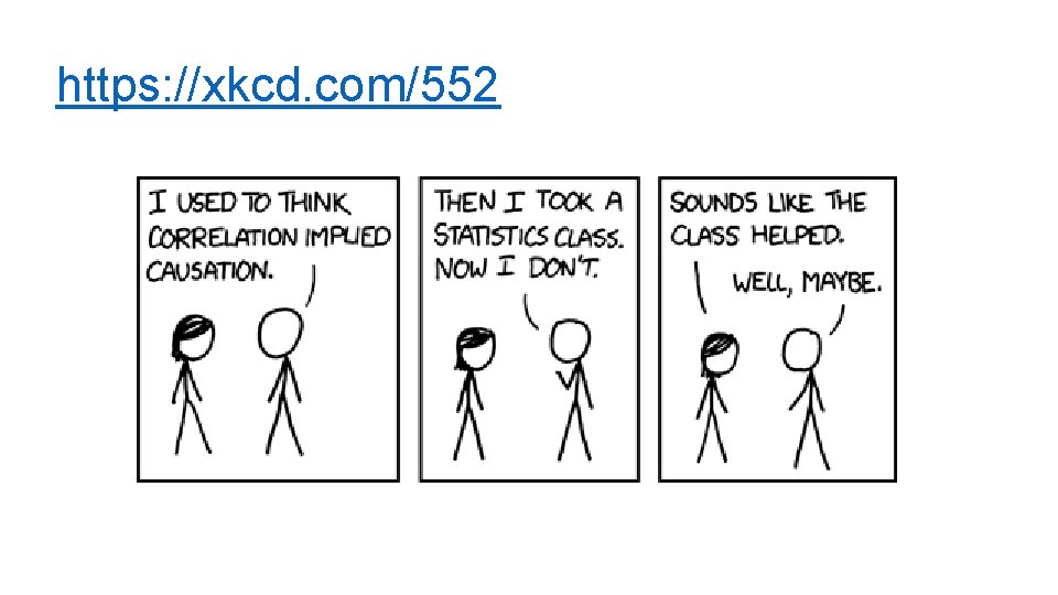
https: //xkcd. com/552

Prosecutor’s Fallacy Ø The probability of 1 in a trillion was computed assuming that the result was due to chance variation. Ø We computed the chance of getting a result as extreme as the one observed, under this assumption. Ø If very rare (tiny probability), we conclude that it is not reasonable to think that random variation is the cause. Ø This logic says nothing about other causes

Prosecutor’s Fallacy – slippery logic C I G Ø Suppose Gilbert is innocent and the deaths behave in a chance-like way. The probability is less than 1 in a trillion that you would see so many excess deaths on Gilbert’s shifts. O L E S Ø If Gilbert is innocent, then it would be almost impossible to get so many excess deaths. L A F Ø With this many excess deaths, the chance is less than one in a trillion that Gilbert is innocent.

Conclusion Ø It is very easy to be tempted by the false logic (that the probability is the chance of innocence). Ø Judge ruled that statistical evidence should not be allowed at trial. Ø Jury found Gilbert guilty on 3 counts of first-degree murder and 2 counts of attempted murder. Ø Jury voted 8 -4 for a death penalty. Ø Gilbert was given life in prison without possibility of parole.

Hypothesis Testing Ø Null Model: Probability model for explaining the chance process for generating the data (the Devil’s advocate process) Ø Test Statistic: summary of data, under the null model it has a sampling distribution Ø Null Hypothesis: Any deviation from what is expected is due to chance variability described by the null model. Ø Alternative Hypothesis: An alternative to the null hypothesis. This may be a simple as “The difference is real”.

Hypothesis Testing Ø p-value: Chance of an outcome as rare or even more rare than the one observed, under the assumptions of the null model. Ø If the p-value is very small, we reject the explanation of chance variability and say that we are convinced that “there is something going on” Ø Depending on the circumstances of the data collection, we may be able to make a stronger statement about the cause.

Hypothesis Testing Ø We have not proven that the null model is false. Ø Our observed test statistic is inconsistent with what the null predicts, then the data are inconsistent with the null. So we reject the null hypothesis. Ø If our observed test statistic is consistent with what the null predicts, we can’t reject the null hypothesis. This and next few slides: A. Adikhari, Data 8

“Inconsistent” What does “inconsistent” mean? ?

“Inconsistent”: the conventions “Inconsistent”: The test statistic is in the tail of the null distribution. “In the tail, ” first convention: ØThe area in the tail is less than 5%. Ø The result is “statistically significant. ” “In the tail, ” second convention: ØThe area in the tail is less than 1%. Ø The result is “highly statistically significant. ”

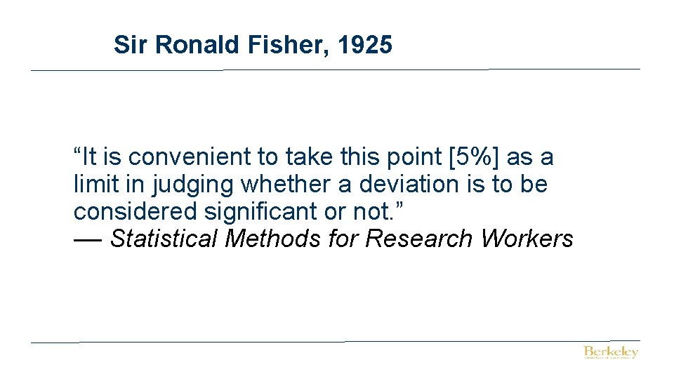
Sir Ronald Fisher, 1925 “It is convenient to take this point [5%] as a limit in judging whether a deviation is to be considered significant or not. ” –– Statistical Methods for Research Workers

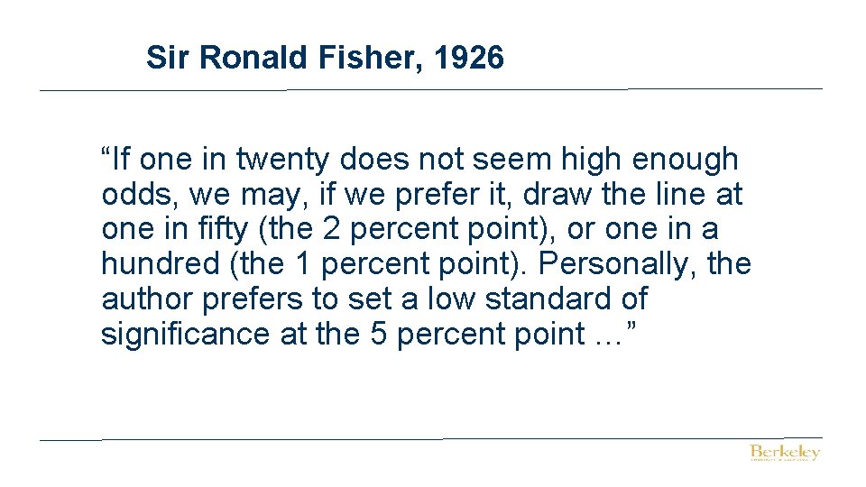
Sir Ronald Fisher, 1926 “If one in twenty does not seem high enough odds, we may, if we prefer it, draw the line at one in fifty (the 2 percent point), or one in a hundred (the 1 percent point). Personally, the author prefers to set a low standard of significance at the 5 percent point …”

K. Gilbert case - references Ø Statistics in the courtroom: United States v. Kristen Gilbert, by G. Cobb and S. Gehlbach. STATS: The magazine for students of statistics, 41: 3 -8. Ø https: //math. buffalostate. edu/~wilsondc/MED 588/Kristen. Gilbert. pdf Ø https: //en. wikipedia. org/wiki/Kristen_Gilbert

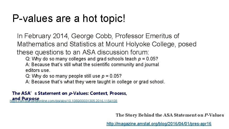
P-values are a hot topic! In February 2014, George Cobb, Professor Emeritus of Mathematics and Statistics at Mount Holyoke College, posed these questions to an ASA discussion forum: Q: Why do so many colleges and grad schools teach p = 0. 05? A: Because that’s still what the scientific community and journal editors use. Q: Why do so many people still use p = 0. 05? A: Because that’s what they were taught in college or grad school. The ASA’s Statement on p-Values: Context, Process, and Purpose https: //amstat. tandfonline. com/doi/abs/10. 1080/00031305. 2016. 1154108 The Story Behind the ASA Statement on P-Values http: //magazine. amstat. org/blog/2016/04/01/pres-apr 16

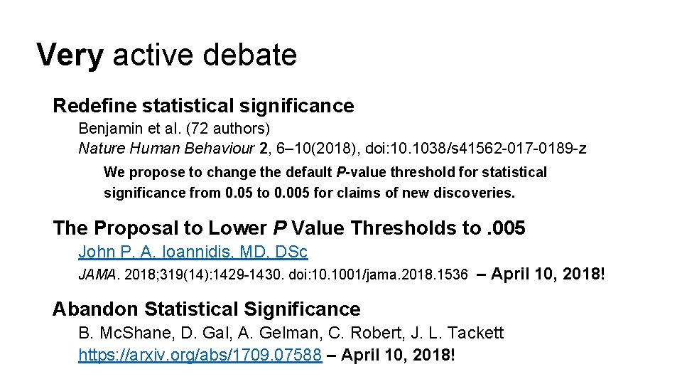
Very active debate Redefine statistical significance Benjamin et al. (72 authors) Nature Human Behaviour 2, 6– 10(2018), doi: 10. 1038/s 41562 -017 -0189 -z We propose to change the default P-value threshold for statistical significance from 0. 05 to 0. 005 for claims of new discoveries. The Proposal to Lower P Value Thresholds to. 005 John P. A. Ioannidis, MD, DSc JAMA. 2018; 319(14): 1429 -1430. doi: 10. 1001/jama. 2018. 1536 – April 10, 2018! Abandon Statistical Significance B. Mc. Shane, D. Gal, A. Gelman, C. Robert, J. L. Tackett https: //arxiv. org/abs/1709. 07588 – April 10, 2018!

P-value calculations A BRIEF DETOUR

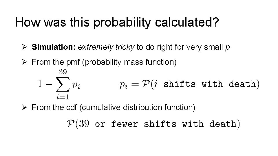
How was this probability calculated? Ø Simulation: extremely tricky to do right for very small p Ø From the pmf (probability mass function) Ø From the cdf (cumulative distribution function)

Simulation was problematic Ø 100, 000 replications of 257 draws produced nothing larger than 26. Ø We can’t estimate this chance as 0 – that’s not useful. We know it is possible. Ø Simulating rare events is hard to do

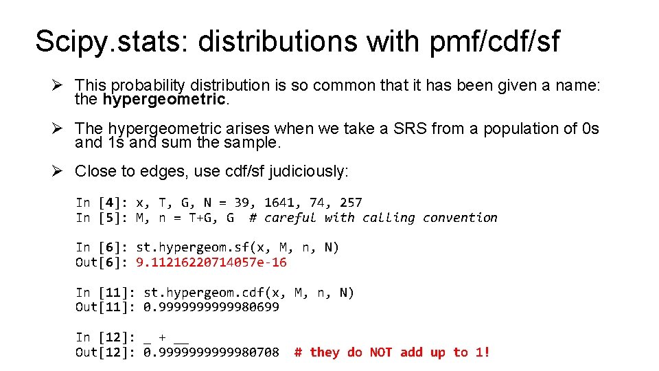
Scipy. stats: distributions with pmf/cdf/sf Ø This probability distribution is so common that it has been given a name: the hypergeometric. Ø The hypergeometric arises when we take a SRS from a population of 0 s and 1 s and sum the sample. Ø Close to edges, use cdf/sf judiciously: In [4]: x, T, G, N = 39, 1641, 74, 257 In [5]: M, n = T+G, G # careful with calling convention In [6]: st. hypergeom. sf(x, M, n, N) Out[6]: 9. 11216220714057 e-16 In [11]: st. hypergeom. cdf(x, M, n, N) Out[11]: 0. 99999980699 In [12]: _ + __ Out[12]: 0. 99999980708 # they do NOT add up to 1!

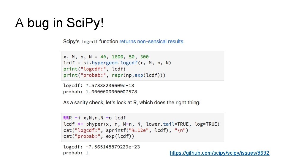
A bug in Sci. Py! https: //github. com/scipy/issues/8692

2. Student Evaluation of Teaching From Boring, Ottoboni, and Stark (2016) “Student evaluations of teaching (mostly) do not measure teaching effectiveness”

Online course 47 Students

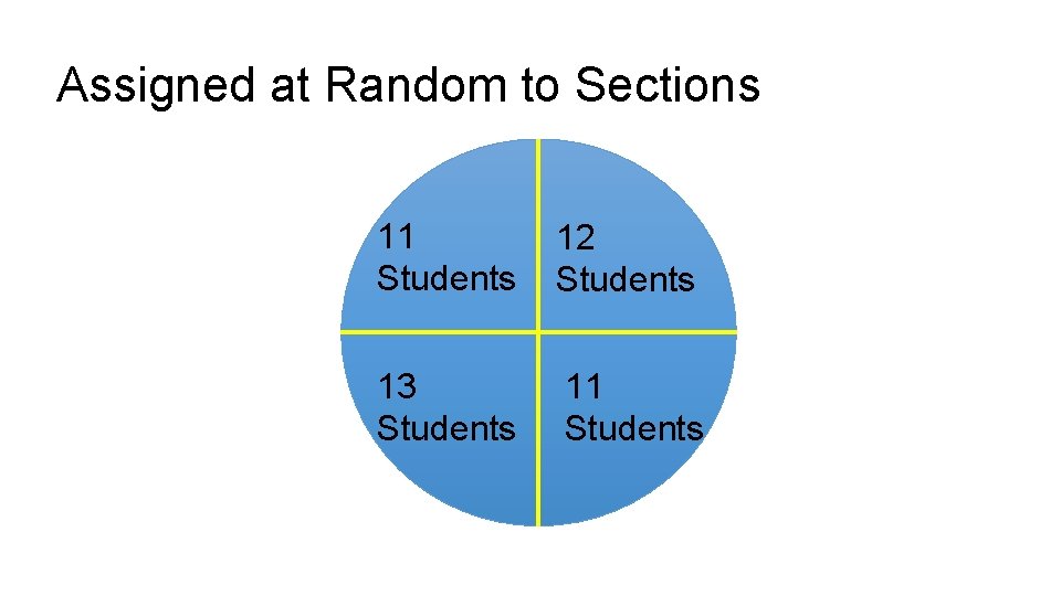
Assigned at Random to Sections 11 Students 12 Students 13 Students 11 Students

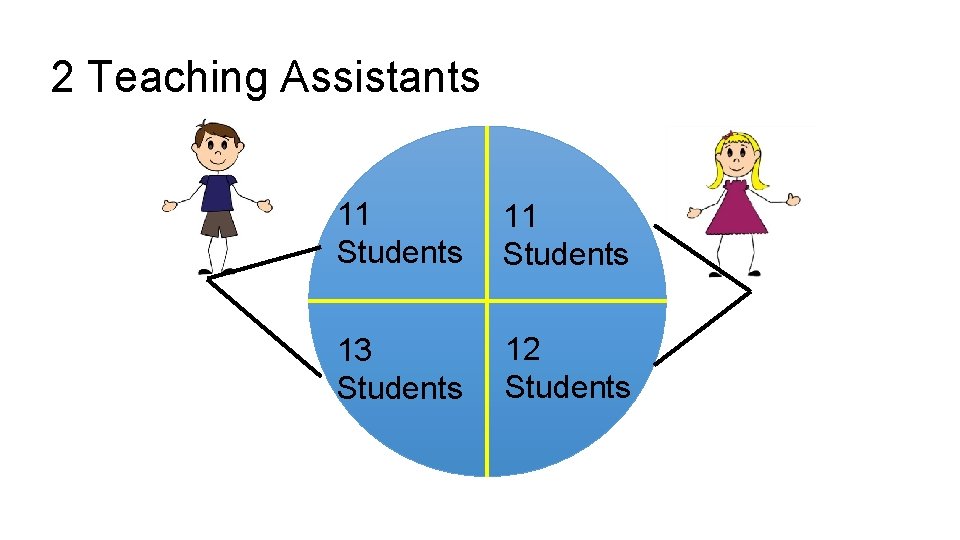
2 Teaching Assistants 11 Students 13 Students 12 Students

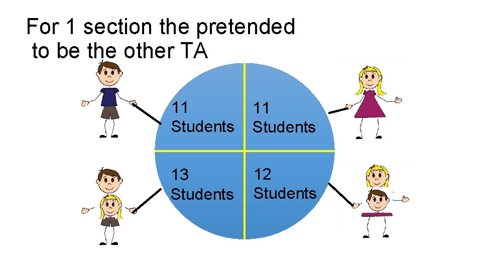
For 1 section the pretended to be the other TA 11 Students 13 Students 12 Students

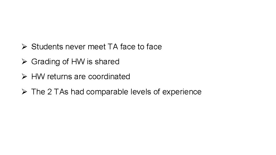
Ø Students never meet TA face to face Ø Grading of HW is shared Ø HW returns are coordinated Ø The 2 TAs had comparable levels of experience

Evaluate the TA on promptness in returning assignment

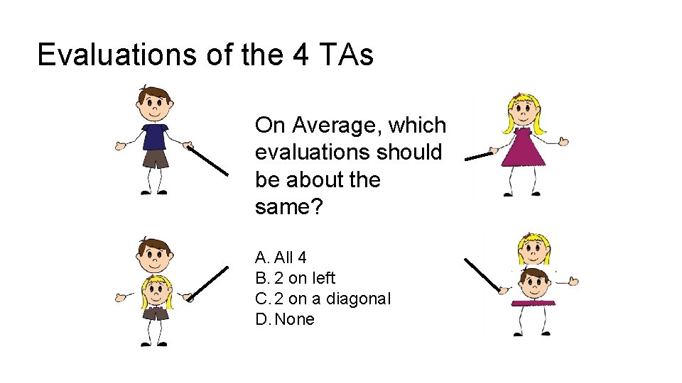
Evaluations of the 4 TAs On Average, which evaluations should be about the same? A. All 4 B. 2 on left C. 2 on a diagonal D. None

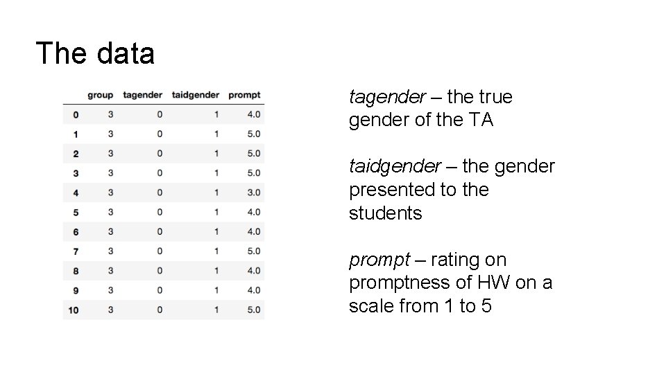
The data tagender – the true gender of the TA taidgender – the gender presented to the students prompt – rating on promptness of HW on a scale from 1 to 5

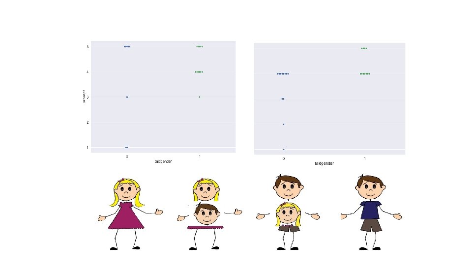
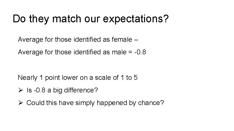
Do they match our expectations? Average for those identified as female – Average for those identified as male = -0. 8 Nearly 1 point lower on a scale of 1 to 5 Ø Is -0. 8 a big difference? Ø Could this have simply happened by chance?

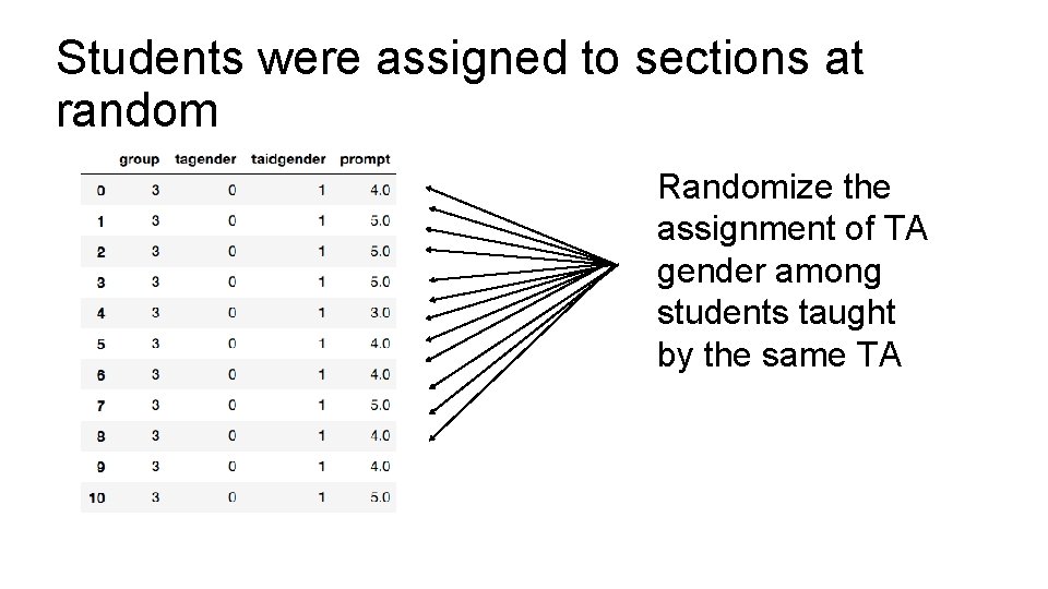
Students were assigned to sections at random Randomize the assignment of TA gender among students taught by the same TA

Ø Randomize the assignment of TA gender among students taught by the same TA Ø These students are taught by the same person Ø The only change is in the perceived gender of the person Ø Presumably the evaluation of the TA should remain unchanged Ø Keep the section sizes the same

Resampling Ø Randomly assign 11 of the female TA’s scores to the identified -female group, Ø Remaining 12 of her scores are assigned to the identified-male group. Ø Randomly assign 13 of the male TA’s scores to the identifiedfemale group and Ø Remaining 11 scores assigned to the identified male group.

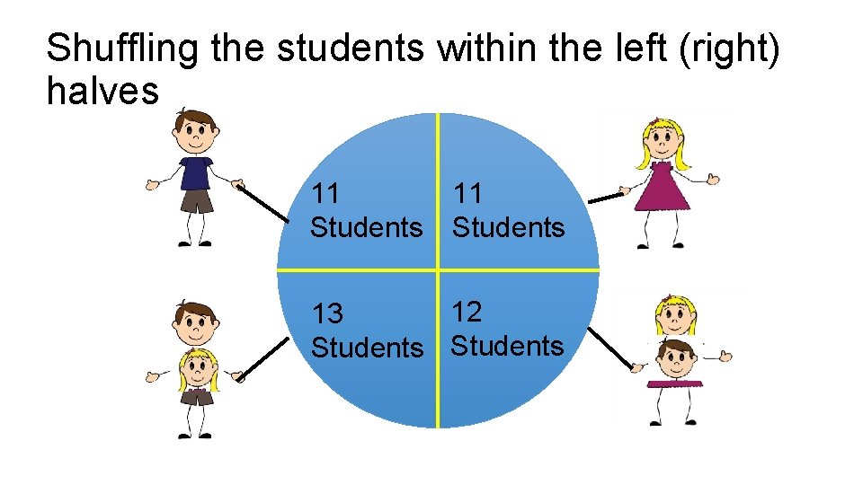
Shuffling the students within the left (right) halves 11 Students 12 13 Students

Ø Compute the difference in average scores for identified-female and identified-male groups. Ø Repeat many times to create an approximate sampling distribution for the difference in average scores for the 2 groups. Ø Use the approximate distribution to estimate the chance of observing -0. 8 or lower

From Boring, Ottoboni & Stark 2016 METHODS (emph. mine) Previous analyses of these data relied on parametric tests based on null hypotheses that do not match the experimental design. For example, the tests assumed that SET of male and female instructors are independent random samples from normally distributed populations with equal variances and possibly different means. As a result, the p-values reported in those studies are for unrealistic null hypotheses and might be misleading. In contrast, we use permutation tests based on the as-if random (French natural experiment) or truly random (US experiment) assignment of students to class sections, with no counterfactual assumption that the students, SET scores, grades, or any other variables comprise random samples from any populations, much less populations with normal distributions.

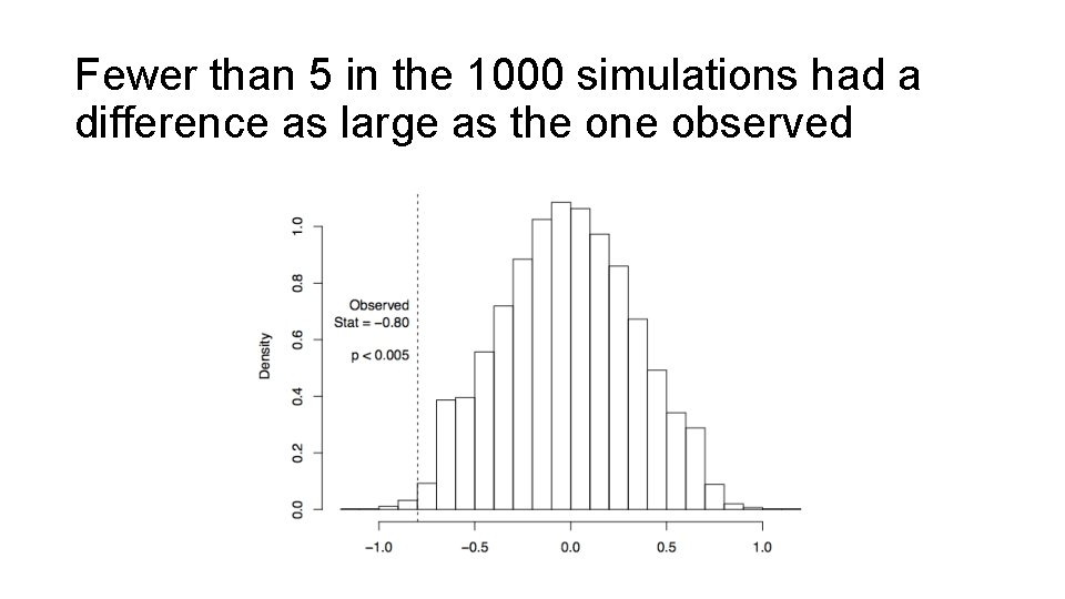
Fewer than 5 in the 1000 simulations had a difference as large as the one observed

T/F Statements Ø The chance is 1 in 200 that the students are biased. Ø The students were assigned to sections at random so this probability calculation is valid Ø Given the protocol for the experimental design, it is reasonable to conclude that the students are gender biased.

Ø These data are from a randomized controlled experiment Ø The randomization and several other aspects of the design made the analysis compelling Ø We must decide whether the evidence is strong enough for us to conclude that there is a gender bias in evaluations

Materials by K. Ottoboni et al. Presentation video @ use. R! 2016 conference Relevant repositories on Git. Hub Ø Code and data for paper: https: //github. com/kellieotto/SET-and-Gender-Bias Ø Permute – Python Library: https: //github. com/statlab/permute Ø Permuter – R Library: https: //github. com/statlab/permuter https: //channel 9. msdn. com/Events/use. R-international-R-User-conference/use. R 2016/Wednesday-June-29 --1048 am-1106 am