Hypothesis testing Chapter 6 Statistics for Marketing Consumer

Hypothesis testing Chapter 6 Statistics for Marketing & Consumer Research Copyright © 2008 - Mario Mazzocchi 1

Sampling and inference 1) 2) 3) 4) 5) Exploit the probabilistic nature of sampling to show statements on the population parameters can be based on sample estimates Consider the degree of uncertainty (level of confidence) in such an operation Build a confidence interval, which is a range of values around the sample mean which is expected to include the true population mean at a given probability (confidence) level Compute the probability associated with a given statement on the population parameters (or parameters from different population) Decide whether the statement is false depending on its probability level (hypothesis testing) Statistics for Marketing & Consumer Research Copyright © 2008 - Mario Mazzocchi 2

Direct and indirect problems • Direct problem – If we knew the population mean and the standard error then we would know the exact probability of any sample mean • Indirect problem – • Confidence interval: Given the sample mean, we can exploit the normal probability curve to find a range of value which will contain the true population mean at a given confidence level • Hypothesis testing: Given the sample mean, we can exploit the normal probability curve to check the probability of an hypothesis on the true mean – then we can decide whether to discard or retain that hypothesis Statistics for Marketing & Consumer Research Copyright © 2008 - Mario Mazzocchi 3

Example • Extract a simple random sample of 100 units out of a population of 400 pub customers • Measure the average expenditure on beer on a sample • The number of potential samples is huge (2. 24*1096) and we observe only one sample • However, if extraction is random, the probability distribution of all sample means is a normal curve centered around the true population mean Statistics for Marketing & Consumer Research Copyright © 2008 - Mario Mazzocchi 4

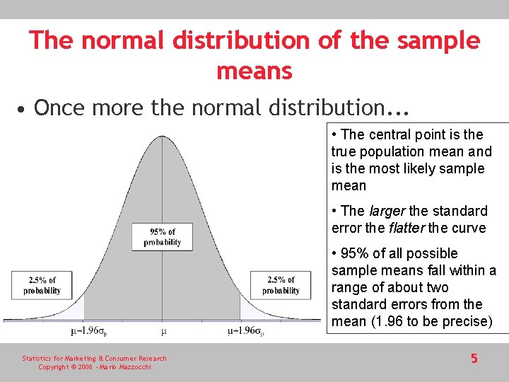
The normal distribution of the sample means • Once more the normal distribution. . . • The central point is the true population mean and is the most likely sample mean • The larger the standard error the flatter the curve • 95% of all possible sample means fall within a range of about two standard errors from the mean (1. 96 to be precise) Statistics for Marketing & Consumer Research Copyright © 2008 - Mario Mazzocchi 5

Indirect problem • We have only one sample mean (x-bar) • 95% of sample means fall within the range • If 100% of the sample means were in that range we could state with certainty that the true mean falls in the range • However, we can affirm that only for 95% of the sample means, thus we refer to a 95% confidence level Statistics for Marketing & Consumer Research Copyright © 2008 - Mario Mazzocchi 6

Confidence level If the single. ONLY sample we. SAMPLE extract. MEANS falls in FALL this range, the – HOWEVER, 95%mean OF THE IN THISthen RANGE true population mean. THAT is also in the interval between THUS WE CAN STATE THEincluded TRUE POPULATION MEAN IS INCLUDED IN THE AND and. INTERVAL BETWEEN. In fact, even if we get one of the. WITH A 95%it. CONFIDENCE extremes, will still be at. LEVEL a distance of 1. 96 sm from m Statistics for Marketing & Consumer Research Copyright © 2008 - Mario Mazzocchi

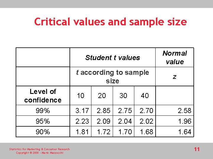
Confidence levels and critical values • The critical value 1. 96 sm corresponds to a probability of 95%, but it is possible to know exact critical values for any confidence level • For example, if we want a 99% confidence level, the critical value based on the normal curve is 2. 58 sm • Most packages including Microsoft Excel allow computation of critical values Statistics for Marketing & Consumer Research Copyright © 2008 - Mario Mazzocchi 8

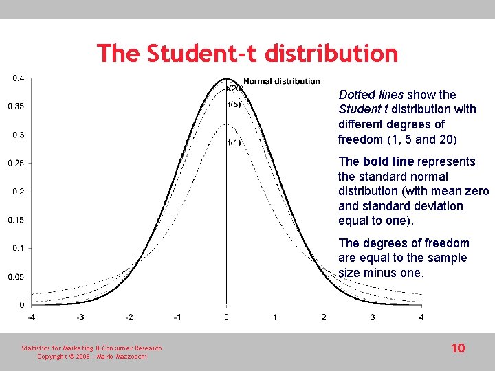
A further complication • The standard error of the mean sm is unknown (sample estimate) • This adds some further uncertainty on the top of the sampling error • Hence, we use an approximation of the normal distribution which is more conservative, is flatter and assigns higher probabilities to the tails (extreme values) compared to the normal distribution • This distribution is the so-called Student-t distribution and its critical values are different from those of the normal distribution Statistics for Marketing & Consumer Research Copyright © 2008 - Mario Mazzocchi 9

The Student-t distribution Dotted lines show the Student t distribution with different degrees of freedom (1, 5 and 20) The bold line represents the standard normal distribution (with mean zero and standard deviation equal to one). The degrees of freedom are equal to the sample size minus one. Statistics for Marketing & Consumer Research Copyright © 2008 - Mario Mazzocchi 10

Critical values and sample size Level of confidence 99% 95% 90% Statistics for Marketing & Consumer Research Copyright © 2008 - Mario Mazzocchi Student t values Normal value t according to sample size z 10 20 30 40 3. 17 2. 23 1. 81 2. 85 2. 09 1. 72 2. 75 2. 04 1. 70 2. 02 1. 68 2. 58 1. 96 1. 64 11

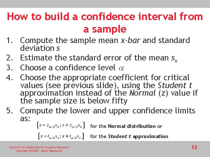
How to build a confidence interval from a sample 1. Compute the sample mean x-bar and standard deviation s 2. Estimate the standard error of the mean sx 3. Choose a confidence level a 4. Choose the appropriate coefficient for critical values (see previous slide), using the Student t approximation instead of the Normal (z) value if the sample size is below fifty 5. Compute the lower and upper confidence limits as: for the Normal distribution or for the Student t approximation Statistics for Marketing & Consumer Research Copyright © 2008 - Mario Mazzocchi 12

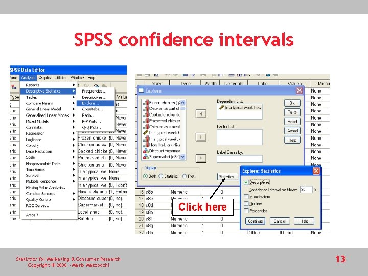
SPSS confidence intervals Click here Statistics for Marketing & Consumer Research Copyright © 2008 - Mario Mazzocchi 13

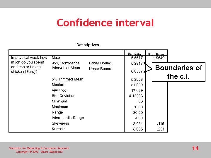
Confidence interval Boundaries of the c. i. Statistics for Marketing & Consumer Research Copyright © 2008 - Mario Mazzocchi 14

Hypothesis testing (HT) • HT is a form of inference • HT is a statistical tool to decide whether to reject or not a statement about the target population on the basis of statistics computed on sample • This is only possible if the sampling distribution is known! Statistics for Marketing & Consumer Research Copyright © 2008 - Mario Mazzocchi 15

Example (Trust data-set) • The sample mean expenditure for chicken is £ 5. 67 • Considering only the sub-sample of those belonging to consumer organizations the mean is £ 5. 04 • May we safely conclude that those who belong to consumer organizations spend less? • This depends on the precision of the estimates. • the upper limit of the 99% confidence interval of the sub-sample of respondents associated to consumer organizations is 6. 84 • the upper limit of the confidence interval for the overall sample is 6. 18 • There is a chance that those who belong to consumer organization actually spend more than other people • Statistical tests based on the sample help in deciding whether the hypothesis should be rejected; for example, that there is no difference between respondents who belong to a consumer organization and those who don’t. Statistics for Marketing & Consumer Research Copyright © 2008 - Mario Mazzocchi 16

Hypothesis testing • The difference between the two means follows a known statistical distribution • If the hypothesis of mean equality is true, the difference between the two means should be zero • The actual difference is it is £ 0. 63 (£ 5. 67 minus £ 5. 04), but this difference may be generated by sampling error • When no difference exists at the population level, what is the probability that a sample with a difference of £ 0. 63 is extracted? • If the probability is very high (say 90%) then it is wise not to reject the hypothesis to equality • Instead, a very low probability (e. g. 0. 001%) means that it is very unlikely that the difference is due sampling error, so one should choose to reject the null hypothesis and conclude that belonging to a consumer organization actually makes a difference on chicken expenditure. Statistics for Marketing & Consumer Research Copyright © 2008 - Mario Mazzocchi 17

The hypotheses • The initial hypothesis is called the null hypothesis, denoted by H 0 • Contextually, the researcher sets an alternative hypothesis (H 1) which is complementary to H 0 and remains valid if H 0 is rejected. • Two-tailed tests are those where the alternative hypothesis can go in either direction • When the alternative hypothesis is formulated in a unique direction (for example m>6), the test is one-tailed Statistics for Marketing & Consumer Research Copyright © 2008 - Mario Mazzocchi 18

Significance and confidence • The threshold probability level below which the null hypothesis is rejected is the significance level arbitrarily set by the researcher (usually at the 5% or 1% level). • It is denoted by a and its complementary 1 -a is the confidence level of a test • The smaller the significance level the smaller the rejection region, (which is the set of values that leads to rejection of the hypothesis) and the larger is the acceptance region, (which is the set of values that lead to non-rejection of the hypothesis) Statistics for Marketing & Consumer Research Copyright © 2008 - Mario Mazzocchi 19

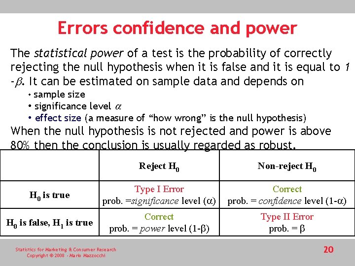
Errors confidence and power The statistical power of a test is the probability of correctly rejecting the null hypothesis when it is false and it is equal to 1 -b. It can be estimated on sample data and depends on • sample size • significance level a • effect size (a measure of “how wrong” is the null hypothesis) When the null hypothesis is not rejected and power is above 80% then the conclusion is usually regarded as robust. Reject H 0 Non-reject H 0 is true Type I Error prob. =significance level (a) Correct prob. = confidence level (1 -a) H 0 is false, H 1 is true Correct prob. = power level (1 -b) Type II Error prob. = b Statistics for Marketing & Consumer Research Copyright © 2008 - Mario Mazzocchi 20

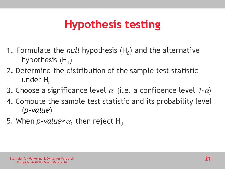
Hypothesis testing 1. Formulate the null hypothesis (H 0) and the alternative hypothesis (H 1) 2. Determine the distribution of the sample test statistic under H 0 3. Choose a significance level a (i. e. a confidence level 1 -a) 4. Compute the sample test statistic and its probability level (p-value) 5. When p-value<a, then reject H 0 Statistics for Marketing & Consumer Research Copyright © 2008 - Mario Mazzocchi 21

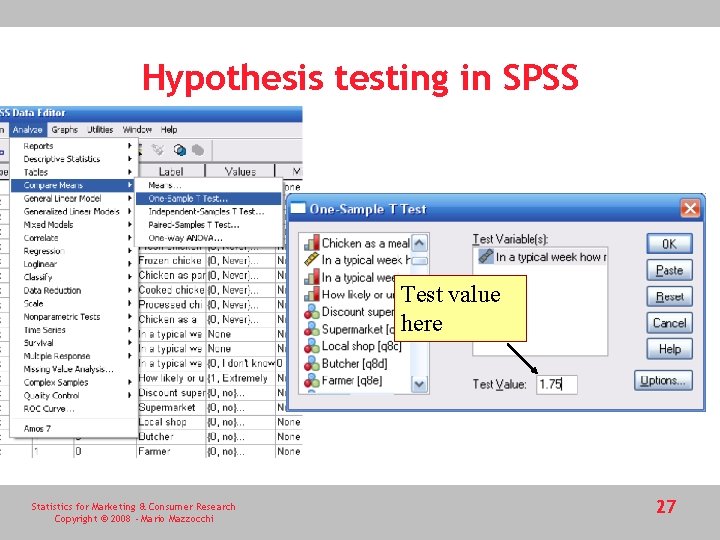
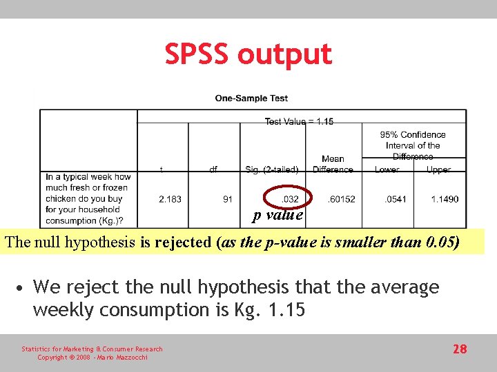
One mean test • The null hypothesis is made on the population mean • Example: • UK Department of Environment, Food and Rural Affairs (DEFRA) figure on average weekly household chicken consumption: 1. 15 Kg • UK household average in the Trust data-set: 1. 75 Kg on 92 respondents • The DEFRA figure is likely to be more representative; we test the hypothesis that the population mean is actually 1. 15 Null H 0: m = 1. 15 versus the alternative H 1: m ≠ 1. 15 Statistics for Marketing & Consumer Research Copyright © 2008 - Mario Mazzocchi 22

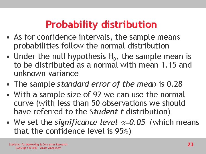
Probability distribution • As for confidence intervals, the sample means probabilities follow the normal distribution • Under the null hypothesis H 0, the sample mean is to be distributed as a normal with mean 1. 15 and unknown variance • The sample standard error of the mean is 0. 28 • With a sample size of 92 we can use the normal curve (with less than 50 observations we should have referred to the Student t distribution) • We set the significance level a=0. 05 (which means that the confidence level is 95%) Statistics for Marketing & Consumer Research Copyright © 2008 - Mario Mazzocchi 23

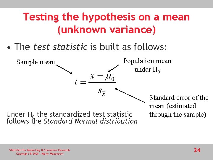
Testing the hypothesis on a mean (unknown variance) • The test statistic is built as follows: Sample mean Population mean under H 0 Under H 0 the standardized test statistic follows the Standard Normal distribution Statistics for Marketing & Consumer Research Copyright © 2008 - Mario Mazzocchi Standard error of the mean (estimated through the sample) 24

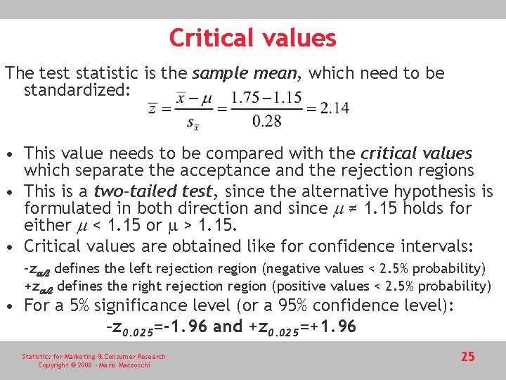
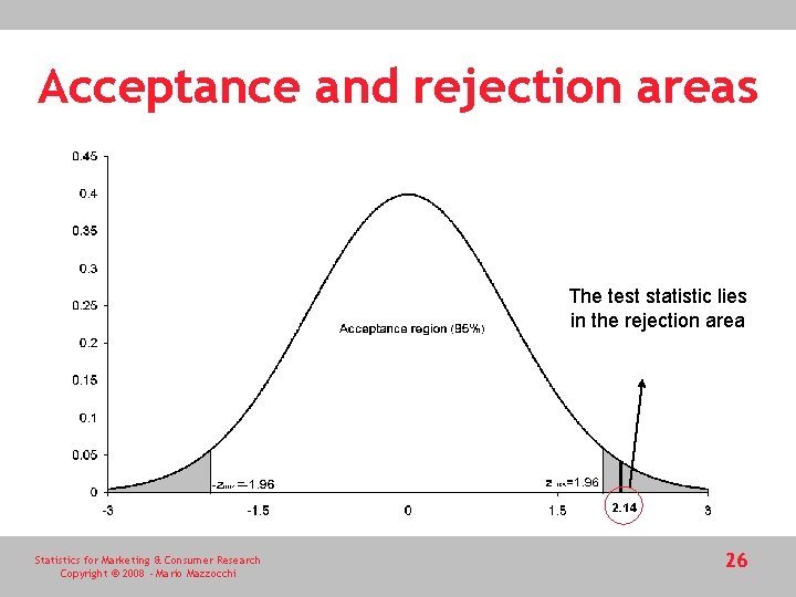
Critical values The test statistic is the sample mean, which need to be standardized: • This value needs to be compared with the critical values which separate the acceptance and the rejection regions • This is a two-tailed test, since the alternative hypothesis is formulated in both direction and since m ≠ 1. 15 holds for either m < 1. 15 or m > 1. 15. • Critical values are obtained like for confidence intervals: -za/2 defines the left rejection region (negative values < 2. 5% probability) +za/2 defines the right rejection region (positive values < 2. 5% probability) • For a 5% significance level (or a 95% confidence level): –z 0. 025=-1. 96 and +z 0. 025=+1. 96 Statistics for Marketing & Consumer Research Copyright © 2008 - Mario Mazzocchi 25

Acceptance and rejection areas The test statistic lies in the rejection area Statistics for Marketing & Consumer Research Copyright © 2008 - Mario Mazzocchi 26

Hypothesis testing in SPSS Test value here Statistics for Marketing & Consumer Research Copyright © 2008 - Mario Mazzocchi 27

SPSS output p value The null hypothesis is rejected (as the p-value is smaller than 0. 05) • We reject the null hypothesis that the average weekly consumption is Kg. 1. 15 Statistics for Marketing & Consumer Research Copyright © 2008 - Mario Mazzocchi 28

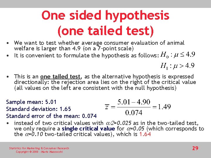
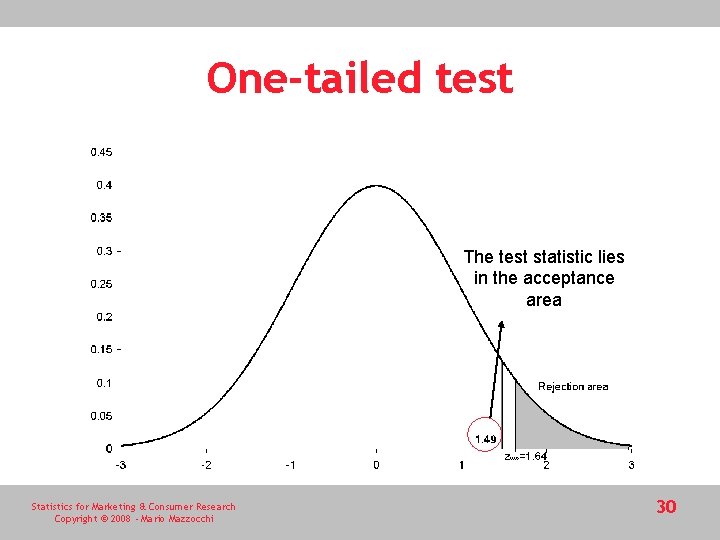
One sided hypothesis (one tailed test) • We want to test whether average consumer evaluation of animal welfare is larger than 4. 9 (on a 7 -point scale) • It is convenient to formulate the hypothesis as follows: • This is an one tailed test, as the alternative hypothesis is expressed directionally: the rejection area lies on the right of the critical value (all values on the left are consistent with the null hypothesis) Sample mean: 5. 01 Standard deviation: 1. 65 Standard error of the mean: 0. 074 • instead of two critical values with a/2=0. 025 as in the two-tailed test, we only require a single critical value for a=0. 05 (which corresponds to the a=0. 10 two-tailed critical values), which is 1. 64 Statistics for Marketing & Consumer Research Copyright © 2008 - Mario Mazzocchi 29

One-tailed test The test statistic lies in the acceptance area Statistics for Marketing & Consumer Research Copyright © 2008 - Mario Mazzocchi 30

One mean one-tailed test in SPSS • Exactly like two-tailed tests, but when interpreting the output: – One should only consider values larger than the positive critical value for rejection (or smaller of the negative critical value if the null direction is >) – To get the correct critical value one should consider the a one instead of a/2 (for example, z 0. 05 rather than z 0. 25) – Thus, the critical value for a 5% significance level in a one-tailed test corresponds to the critical value for a 10% two-tailed test. For example z 0. 05=1. 64 – Similarly, when looking at the two-tailed test p-value in SPSS, one should consider a “double” threshold, i. e. reject the null at the 95% level when p>0. 10 (since SPSS always assumes two-tailed tests) Statistics for Marketing & Consumer Research Copyright © 2008 - Mario Mazzocchi 31

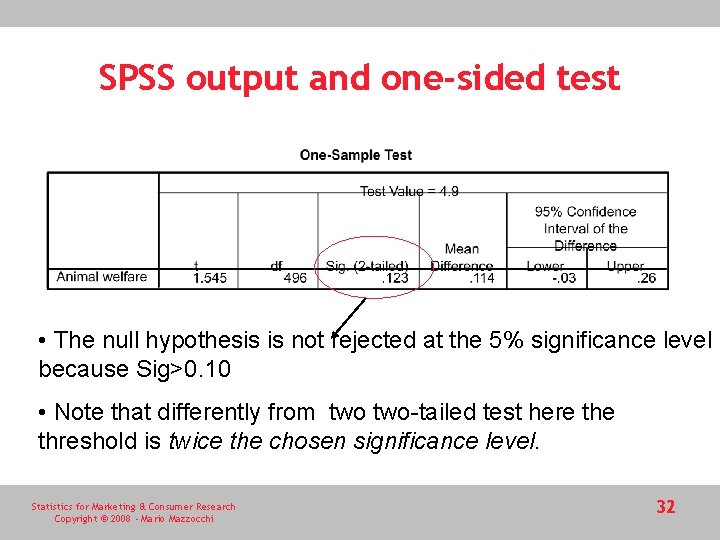
SPSS output and one-sided test • The null hypothesis is not rejected at the 5% significance level because Sig>0. 10 • Note that differently from two-tailed test here threshold is twice the chosen significance level. Statistics for Marketing & Consumer Research Copyright © 2008 - Mario Mazzocchi 32

Test on two means • Tests of equality on two means follow directly from the single-mean test • The difference of two normally distributed sample means is still a normally distributed, provided that the samples are unrelated or paired • The mean of the difference distribution is zero under the null hypothesis of mean equality Statistics for Marketing & Consumer Research Copyright © 2008 - Mario Mazzocchi 33

Unrelated samples • The sampled units belong to different populations and are randomly extracted from each of the population. The key condition is that the sampled units are randomly assigned to the two groups • This excludes the case where: a) a single sample is drawn b) the units are subdivided into two groups according to some variable (gender, living in urban versus rural areas, etc. ) c) the sampling process might have some selection bias creating dependency between the two groups • Most social studies consider the samples to be unrelated if the units are randomly extracted and the groups are mutually exclusive. Statistics for Marketing & Consumer Research Copyright © 2008 - Mario Mazzocchi 34

Related and paired samples • In related samples he same subjects may belong to both groups. • For example, if the same individual is interviewed in two waves, the two samples are said to be related. • Two sub-sets from the sample are generally related (not for stratified sampling) • Paired samples are a special case where exactly the same units appear in both samples • In this case it is possible to compute the difference for each of the sampled units and the result corresponds to a single sample • Matched samples are artificially paired samples, where the two samples are matched according to some characteristics. Statistics for Marketing & Consumer Research Copyright © 2008 - Mario Mazzocchi 35

Example (Trust data-set) • 71% of respondents are female • the targeted population are people in charge of food purchases; males and females in the Trust data-set are associated by the fact that they are responsible for food purchases • This excludes those females and males who are not; any gender comparison is conditional on this external factor • We could not be conclusive in testing – for example – whether males like chicken more than females Statistics for Marketing & Consumer Research Copyright © 2008 - Mario Mazzocchi 36

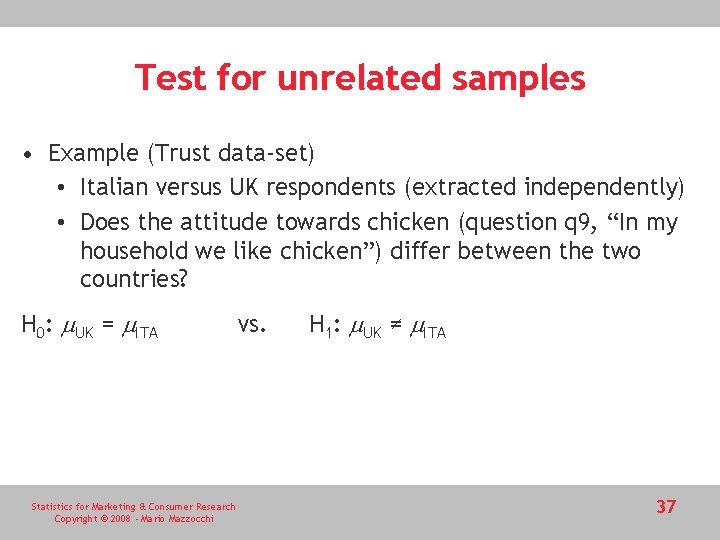
Test for unrelated samples • Example (Trust data-set) • Italian versus UK respondents (extracted independently) • Does the attitude towards chicken (question q 9, “In my household we like chicken”) differ between the two countries? H 0: m. UK = m. ITA Statistics for Marketing & Consumer Research Copyright © 2008 - Mario Mazzocchi vs. H 1: m. UK ≠ m. ITA 37

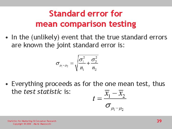
Unrelated samples • The two means are normally distributed • Under the null hypothesis their difference is also normally distributed • Consider the difference variable D = m. UK - m. ITA • The test becomes identical to the one mean test for D = 0 • However, a measure of the standard error for D is necessary Statistics for Marketing & Consumer Research Copyright © 2008 - Mario Mazzocchi 38

Standard error for mean comparison testing • In the (unlikely) event that the true standard errors are known the joint standard error is: • Everything proceeds as for the one mean test, thus the test statistic is: Statistics for Marketing & Consumer Research Copyright © 2008 - Mario Mazzocchi 39

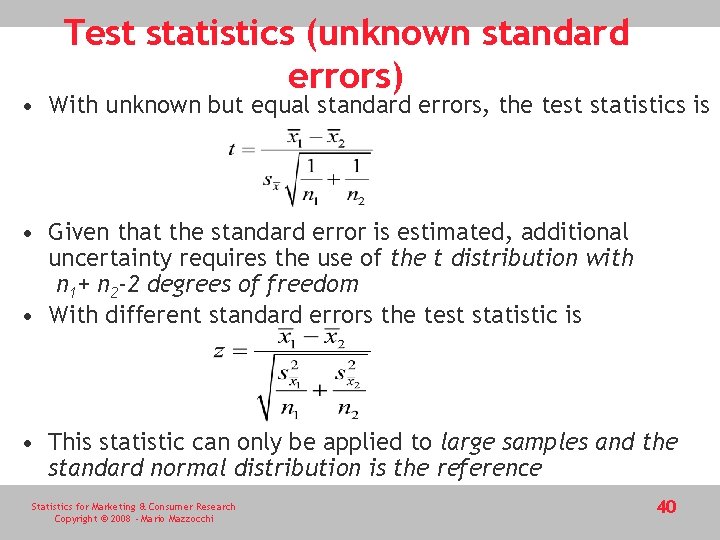
Test statistics (unknown standard errors) • With unknown but equal standard errors, the test statistics is • Given that the standard error is estimated, additional uncertainty requires the use of the t distribution with n 1+ n 2 -2 degrees of freedom • With different standard errors the test statistic is • This statistic can only be applied to large samples and the standard normal distribution is the reference Statistics for Marketing & Consumer Research Copyright © 2008 - Mario Mazzocchi 40

How to decide whether the standard errors are equal or different? • There appropriate hypothesis tests for the equality of two variances (discussed later) • SPSS shows the p-value for the Levene’s test (Brown and Forsythe, 1974) • SPSS provides the outcomes of both test, with and without assuming equality of standard errors. • In most cases these two tests provide consistent outcomes. Statistics for Marketing & Consumer Research Copyright © 2008 - Mario Mazzocchi 41

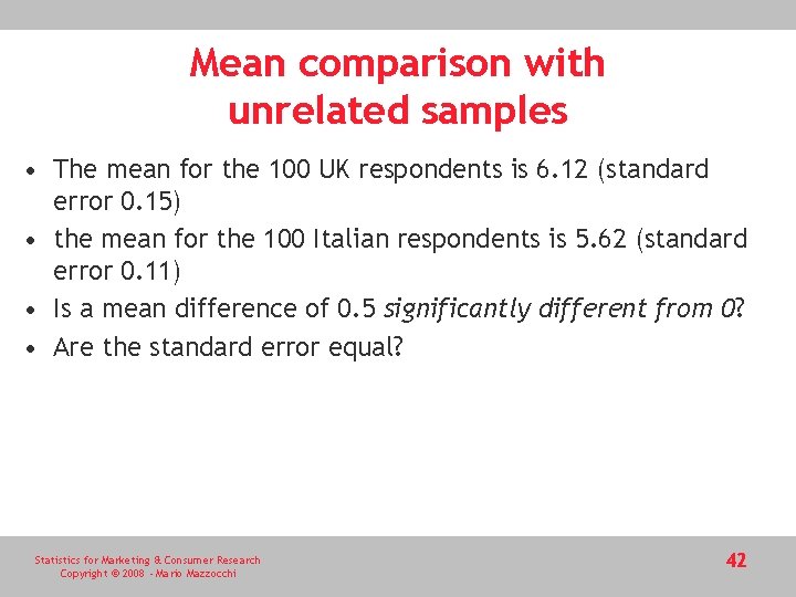
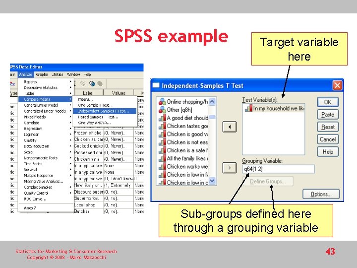
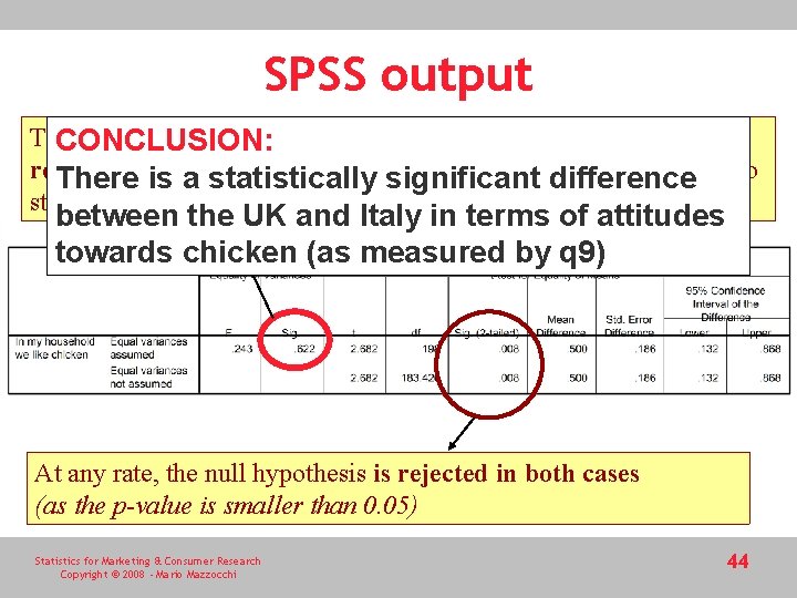
Mean comparison with unrelated samples • The mean for the 100 UK respondents is 6. 12 (standard error 0. 15) • the mean for the 100 Italian respondents is 5. 62 (standard error 0. 11) • Is a mean difference of 0. 5 significantly different from 0? • Are the standard error equal? Statistics for Marketing & Consumer Research Copyright © 2008 - Mario Mazzocchi 42

SPSS example Target variable here Sub-groups defined here through a grouping variable Statistics for Marketing & Consumer Research Copyright © 2008 - Mario Mazzocchi 43

SPSS output The null hypothesis of equality of variance (Levene’s test) is not CONCLUSION: rejected thea 5% s. l. (as p-value is larger thandifference 0. 05), thus the two Thereatis statistically significant standard errors could be regarded as equal between the UK and Italy in terms of attitudes towards chicken (as measured by q 9) At any rate, the null hypothesis is rejected in both cases (as the p-value is smaller than 0. 05) Statistics for Marketing & Consumer Research Copyright © 2008 - Mario Mazzocchi 44

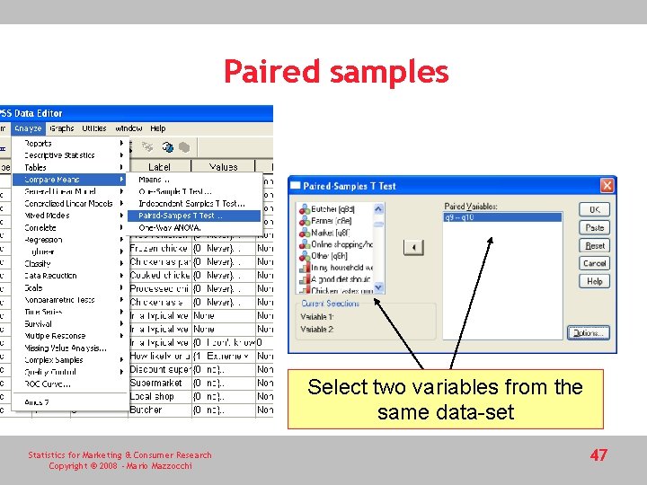
Paired samples • As a second case study, consider the situation where two measures are taken on the same respondents. • For example, all respondents were asked a second question on their general attitude towards chicken, “A good diet should always include chicken” (q 10) • Do the two questions measure the same item (general attitude towards chicken)? • Can we assume that the results are – on average – equal? • In this case the samples are paired and it is possible to compute a difference between the response to q 9 and q 10 for each of the sampled household. • Everything goes back to one mean test discussed earlier Statistics for Marketing & Consumer Research Copyright © 2008 - Mario Mazzocchi 45

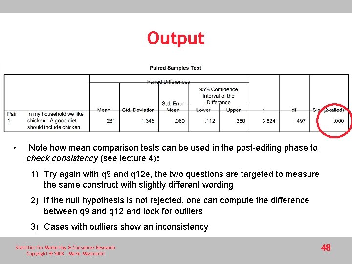
Paired samples • One may compute a third variable for each of the respondent as the difference between q 9 and q 10, then compute the mean and the standard error for this variable • SPSS does this automatically – – mean of 5. 73 for q 9 versus a mean of 5. 50 for q 10 average difference 0. 23 estimated standard error 0. 06. The t test statistic is 3. 84, largely above the two-tailed 99% critical value, • the null hypothesis of mean equality should be rejected. • It is not safe to assume that the two questions are measuring the same construct Statistics for Marketing & Consumer Research Copyright © 2008 - Mario Mazzocchi 46

Paired samples Select two variables from the same data-set Statistics for Marketing & Consumer Research Copyright © 2008 - Mario Mazzocchi 47

Output • Note how mean comparison tests can be used in the post-editing phase to check consistency (see lecture 4): 1) Try again with q 9 and q 12 e, the two questions are targeted to measure the same construct with slightly different wording 2) If the null hypothesis is not rejected, one can compute the difference between q 9 and q 12 and look for outliers 3) Cases with outliers show an inconsistency Statistics for Marketing & Consumer Research Copyright © 2008 - Mario Mazzocchi 48

Other type of tests • Independent samples • Standard t-test (as seen) • Paired samples • It becomes a one-sample t-test • Related samples • Non-parametric tests Statistics for Marketing & Consumer Research Copyright © 2008 - Mario Mazzocchi 49

Related samples tests and non-parametric statistics • Do not require knowledge of the underlying distributions (see Gibbons, 1993 for a good introduction to nonparametric testing). • Non-parametric tests are also used in situations where the variables to be tested are qualitative Statistics for Marketing & Consumer Research Copyright © 2008 - Mario Mazzocchi 50

Non-parametric testing (NPT) • Parametric methods assume knowledge of the distribution (usually normal) and its parameters • Problems: different distributions (income), small sample sizes, etc. • NPT – No prior assumption on the distribution (and its parameters) Statistics for Marketing & Consumer Research Copyright © 2008 - Mario Mazzocchi 51

Some non-parametric tests One group • Runs (Wald-Wolfowitz) • Kolmogorov-Smirnov • Chi-square test • Binomial test • Wilcoxon signed-rank Two groups • Runs (Wald-Wolfowitz) on two groups • Mann-Whitney test (Wilcoxon-rank-sum test) • Kolmogorov-Smirnov on two groups • Wilcoxon paired sample test (on two paired samples) Statistics for Marketing & Consumer Research Copyright © 2008 - Mario Mazzocchi 52

Runs test • On one group • Check whether the order in the sample is random • Check whether observations below and above a cut-off point (e. g. median) follow a random order • On two groups • Check whether observations from two groups follow a random order (after being sorted according to some variable) Statistics for Marketing & Consumer Research Copyright © 2008 - Mario Mazzocchi 53

One-group tests Statistics for Marketing & Consumer Research Copyright © 2008 - Mario Mazzocchi 54

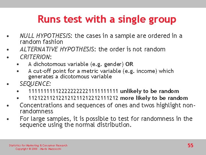
Runs test with a single group • NULL HYPOTHESIS: the cases in a sample are ordered in a random fashion ALTERNATIVE HYPOTHESIS: the order is not random CRITERION: • • • SEQUENCE: • • A dichotomous variable (e. g. gender) OR A cut-off point for a metric variable (e. g. income) which generates a dicotomous variable 111112222211111 unlikely to be random 112122121211212212111212 more likely to be random Concentrations and sequences of ones and twos highlight nonrandomness For large samples, it is possible to test for randomness in the sequence using the normal distribution. Statistics for Marketing & Consumer Research Copyright © 2008 - Mario Mazzocchi 55

Kolmogorov-Smirnov • The null hypothesis is that a random sample is drawn from a (user specified) given distribution • SPSS allows to test whether a variable is distributed according to a normal distribution, a Poisson curve, a uniform or an exponential distribution • Once the distribution and its parameters are known, it becomes possible to estimate the population parameters Statistics for Marketing & Consumer Research Copyright © 2008 - Mario Mazzocchi 56

Chi-square test • Compare the frequency of the observed distribution with the expected frequency from a theoretical distribution (e. g. the normal curve) • The more different are the frequencies, the less likely it is that the empirical observations come from theoretical distribution • The Chi-square statistics synthesizes the distance between the observed and expected frequencies and is compared to critical values from the Chi-square distribution Statistics for Marketing & Consumer Research Copyright © 2008 - Mario Mazzocchi 57

Binomial test • Applied to dichotomous variables, e. g. gender (males and females) • NULL HYPOTHESIS: the proportion of males and females in the sample is imputable to sampling error only • E. g. if we get 71% females and 29% males in the trust dataset, could this depend on sampling error only? • Assuming a 50%-50% true distribution between males and females, a 71 -29 outcome leads to rejection of the null hypothesis Statistics for Marketing & Consumer Research Copyright © 2008 - Mario Mazzocchi 58

Wilcoxon signed rank test • Non-parametric correspondent of the one-mean t-test • NULL HYPOTHESIS: the median (or the difference between two medians) is equal to some specified value, provided that the distribution is symmetric • CRITERION: based on ranking, which consists of assigning increasing discrete values one, two, etc. to the cases once they have been sorted in ascending order according to the variable to be tested • The observations which differ from the hypothesized median are ranked according to their distance from the median • Ranks above and below the assumed median are summated to build the test statistic Statistics for Marketing & Consumer Research Copyright © 2008 - Mario Mazzocchi 59

Two groups tests Statistics for Marketing & Consumer Research Copyright © 2008 - Mario Mazzocchi 60

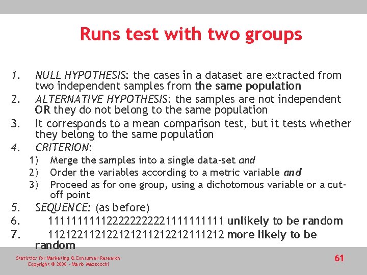
Runs test with two groups 1. 2. 3. 4. NULL HYPOTHESIS: the cases in a dataset are extracted from two independent samples from the same population ALTERNATIVE HYPOTHESIS: the samples are not independent OR they do not belong to the same population It corresponds to a mean comparison test, but it tests whether they belong to the same population CRITERION: 1) 2) 3) 5. 6. 7. Merge the samples into a single data-set and Order the variables according to a metric variable and Proceed as for one group, using a dichotomous variable or a cutoff point SEQUENCE: (as before) 111112222211111 unlikely to be random 112122121211212212111212 more likely to be random Statistics for Marketing & Consumer Research Copyright © 2008 - Mario Mazzocchi 61

Mann-Whitney test • Also known as the Wilcoxon-rank-sum test • ASSUMPTION: the two samples are random and come from population that follow the same distribution apart from a translation k • NULL HYPOTHESIS: k=0 (which means that the samples are extracted from the same population) • The null here is stronger than the null of mean equality Statistics for Marketing & Consumer Research Copyright © 2008 - Mario Mazzocchi 62

Example (Trust) (1) • • • Trust in the European food safety authority for French (F) and German (G) respondents (measured on a one to seven scale) Trust of Germans = Trust of French + k NULL HYPOTHESIS H 0: k= 0 Statistics for Marketing & Consumer Research Copyright © 2008 - Mario Mazzocchi 63

Trust (2) 1. 2. 3. 4. 5. All cases are ranked by trust level independently from the country and a rank number is assigned Ranks for each group (F and G) are summated The sums are compared (allowing for different group sizes) through the U statistic The U statistic is based on the frequency with whom the first sample has a higher rank than the second sample If the two samples come from the same distribution the frequency should be random (similarly for the Run test) Statistics for Marketing & Consumer Research Copyright © 2008 - Mario Mazzocchi 64

Other tests Kolmogorov-Smirnov for two groups • Two distributions are compared, instead of simply comparing theoretical distribution with the empirical one Wilcoxon paired sample test • Wilcoxon signed rank test on the median difference between the two samples provided that the differences are symmetrically distributed Statistics for Marketing & Consumer Research Copyright © 2008 - Mario Mazzocchi 65

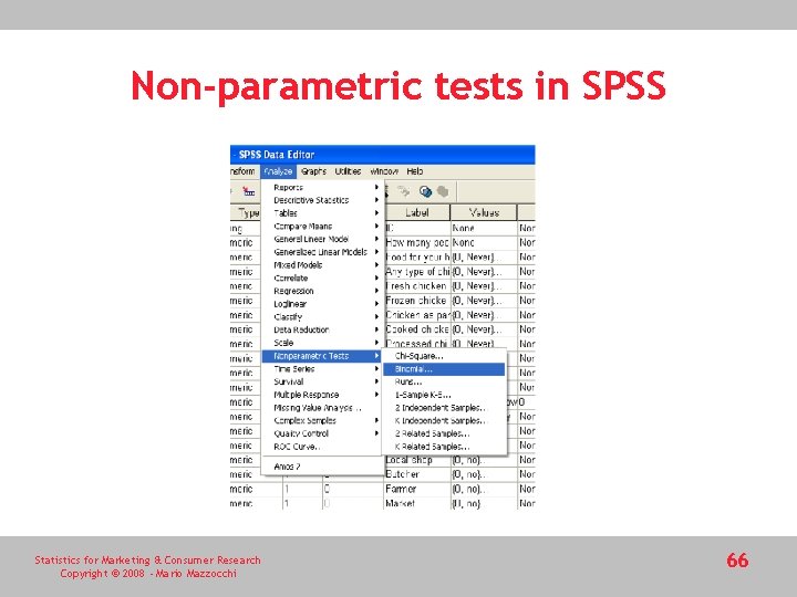
Non-parametric tests in SPSS Statistics for Marketing & Consumer Research Copyright © 2008 - Mario Mazzocchi 66

Other tests • Test on proportions • Proceed like for means • For large samples they correspond to test on means (use the normal distribution) • Test on variances • F-test for the equality of variances • Levene’s F-test Statistics for Marketing & Consumer Research Copyright © 2008 - Mario Mazzocchi 67

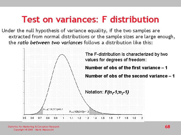
Test on variances: F distribution Under the null hypothesis of variance equality, if the two samples are extracted from normal distributions or the sample sizes are large enough, the ratio between two variances follows a distribution like this: The F-distribution is characterized by two values for degrees of freedom: Number of obs of the first variance – 1 Number of obs of the second variance – 1 Notation: F(n 1 -1; n 2 -1) Statistics for Marketing & Consumer Research Copyright © 2008 - Mario Mazzocchi 68

F-test • Note that the F distribution only includes positive value; it is nonsymmetrical and for two-tailed tests the critical values are defined in a slightly different manner when compared to the t and normal distributions • For a given significance level a, the critical value for the right rejection region (the first variance is larger than the second) is denoted by Fa/2 as usual, since we want to exclude F values larger than Fa/2 because their probability is below a/2. • Instead, the critical value for the left rejection area is denoted as F 1 -a/2 , since we set the probability that F is larger than the critical value to 1 -a/2, which means that the probability that F is smaller than the critical value is actually a/2, as desired. • This difference is also relevant to one-tailed test where the alternative hypothesis is s 1 < s 2, where the critical value will be F 1 -a Statistics for Marketing & Consumer Research Copyright © 2008 - Mario Mazzocchi 69

Example (Trust data) • Is the variance in chicken consumption for males equal to the variance for females? H 0 : s. M = s. F vs H 1: s. M ≠ s. F • Variance males: 0. 87 • Variance females: 2. 60 • F-statistic: 0. 87/2. 60=0. 33 • Critical values: F 0. 975(129, 313)=0. 74 F 0. 025(129, 313)=1. 33 • The null hypothesis is rejected Statistics for Marketing & Consumer Research Copyright © 2008 - Mario Mazzocchi 70

Other tests on variances • The standard F test is valid under the assumption of normal distribution of the populations • Generalization for non-normal populations (SPSS and SAS): • Levene’s test for homogeneity of variances (slightly different F statistic). • Levene’s test can be biased by the presence of outliers Statistics for Marketing & Consumer Research Copyright © 2008 - Mario Mazzocchi 71