Hypothesis Testing Berlin Chen Department of Computer Science

Hypothesis Testing Berlin Chen Department of Computer Science & Information Engineering National Taiwan Normal University Reference: 1. W. Navidi. Statistics for Engineering and Scientists. Chapter 6 & Teaching Material

Introduction - Scenario for Hypothesis Test • Recall the Example in Chapter 5 about Microdrills – Our sample had a mean of 12. 68 and standard deviation of 6. 83 – Let us assume that the main question is: Whether or not the population mean lifetime is greater than 11 ? • We can address this by examining the value of the sample mean • We see that our sample mean is larger than 11, but because of uncertainty in the means, this does not guarantee that > 11 – We would like to know just how certain we can be that > 11 • A confidence interval is not quite what we need – The statement “ > 11” is a hypothesis about the population mean – To determine just how certain we can be that a hypothesis is true, we must perform a hypothesis test (假設檢定) 2

Large-Sample Test for a Population Mean • The null hypothesis (虛擬假設) – (In most cases) Says that the effect indicated by the sample is due only to random variation between the sample and the population. We denote this with H 0 • The alternate hypothesis (對立假設) – Says that the effect indicated by the sample is real, in that it accurately represents the whole population. We denote this with H 1 • In performing a hypothesis test, we essentially put the null hypothesis on trial – We begin by assuming that H 0 is true just as we begin a trial by assuming a defendant to be innocent – The random sample provides the evidence – The hypothesis test involves measuring the strength of the disagreement between the sample and H 0 to produce a number between 0 and 1, called a P-value 3

P-Value • The P-value measures the plausibility of H 0 • The smaller the P-value, the stronger the evidence is against H 0 • If the P-value is sufficiently small, we may be willing to abandon our assumption that H 0 is true and believe H 1 instead • This is referred to as rejecting the null hypothesis 4

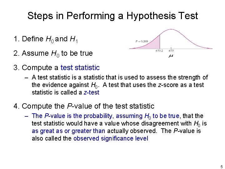
Steps in Performing a Hypothesis Test 1. Define H 0 and H 1 2. Assume H 0 to be true 3. Compute a test statistic – A test statistic is a statistic that is used to assess the strength of the evidence against H 0. A test that uses the z-score as a test statistic is called a z-test 4. Compute the P-value of the test statistic – The P-value is the probability, assuming H 0 to be true, that the test statistic would have a value whose disagreement with H 0 is as great as or greater than actually observed. The P-value is also called the observed significance level 5

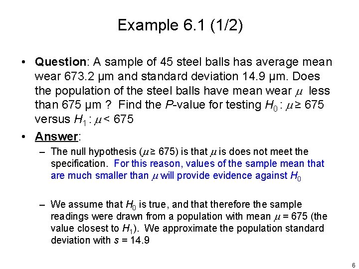
Example 6. 1 (1/2) • Question: A sample of 45 steel balls has average mean wear 673. 2 μm and standard deviation 14. 9 μm. Does the population of the steel balls have mean wear less than 675 μm ? Find the P-value for testing H 0 : ≥ 675 versus H 1 : < 675 • Answer: – The null hypothesis ( ≥ 675) is that is does not meet the specification. For this reason, values of the sample mean that are much smaller than will provide evidence against H 0 – We assume that H 0 is true, and that therefore the sample readings were drawn from a population with mean = 675 (the value closest to H 1). We approximate the population standard deviation with s = 14. 9 6

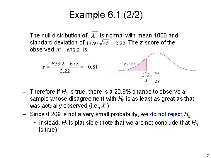
Example 6. 1 (2/2) – The null distribution of standard deviation of observed is is normal with mean 1000 and The z-score of the – Therefore if H 0 is true, there is a 20. 9% chance to observe a sample whose disagreement with H 0 is as least as great as that was actually observed (i. e. , ) – Since 0. 209 is not a very small probability, we do not reject H 0 • Instead, H 0 is plausible (note that we are not conclude that H 0 is true) 7

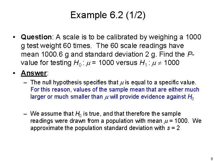
Example 6. 2 (1/2) • Question: A scale is to be calibrated by weighing a 1000 g test weight 60 times. The 60 scale readings have mean 1000. 6 g and standard deviation 2 g. Find the Pvalue for testing H 0 : = 1000 versus H 1 : 1000 • Answer: – The null hypothesis specifies that is equal to a specific value. For this reason, values of the sample mean that are either much larger or much smaller than will provide evidence against H 0 – We assume that H 0 is true, and that therefore the sample readings were drawn from a population with mean = 1000. We approximate the population standard deviation with s = 2 8

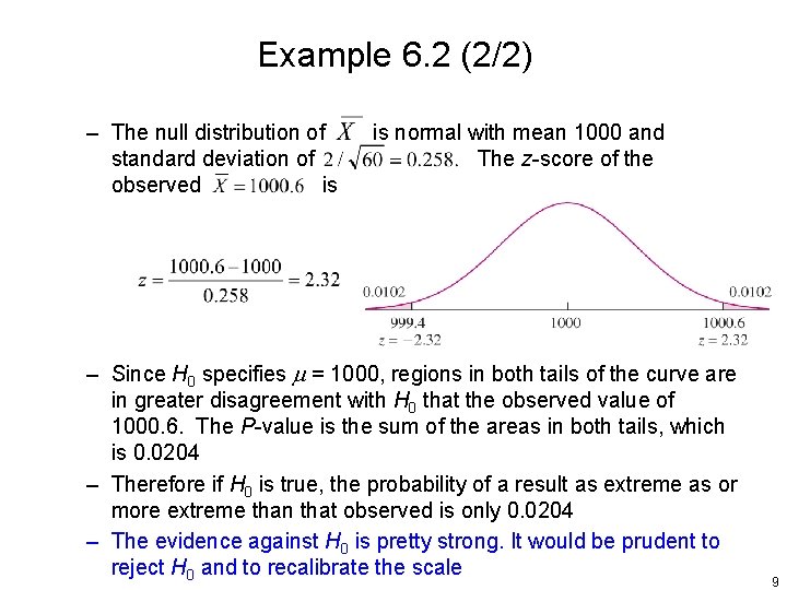
Example 6. 2 (2/2) – The null distribution of standard deviation of observed is is normal with mean 1000 and The z-score of the – Since H 0 specifies = 1000, regions in both tails of the curve are in greater disagreement with H 0 that the observed value of 1000. 6. The P-value is the sum of the areas in both tails, which is 0. 0204 – Therefore if H 0 is true, the probability of a result as extreme as or more extreme than that observed is only 0. 0204 – The evidence against H 0 is pretty strong. It would be prudent to reject H 0 and to recalibrate the scale 9

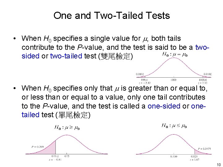
One and Two-Tailed Tests • When H 0 specifies a single value for , both tails contribute to the P-value, and the test is said to be a twosided or two-tailed test (雙尾檢定) • When H 0 specifies only that is greater than or equal to, or less than or equal to a value, only one tail contributes to the P-value, and the test is called a one-sided or onetailed test (單尾檢定) 10

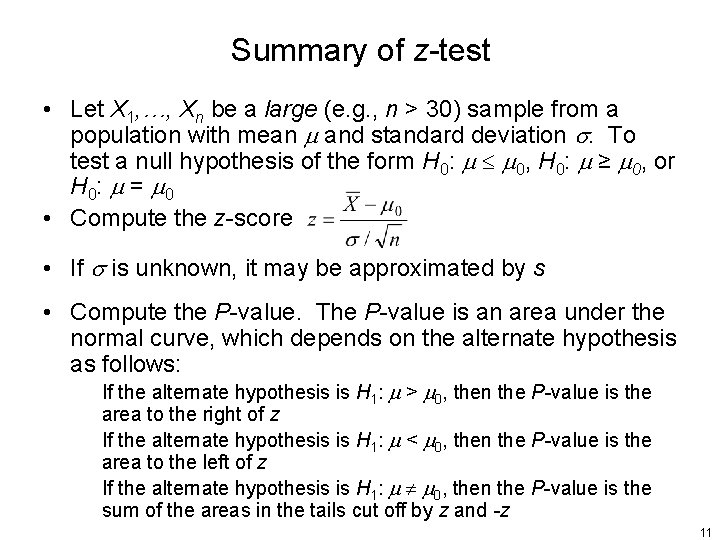
Summary of z-test • Let X 1, …, Xn be a large (e. g. , n > 30) sample from a population with mean and standard deviation . To test a null hypothesis of the form H 0: 0, H 0: ≥ 0, or H 0: = 0 • Compute the z-score • If is unknown, it may be approximated by s • Compute the P-value. The P-value is an area under the normal curve, which depends on the alternate hypothesis as follows: If the alternate hypothesis is H 1: > 0, then the P-value is the area to the right of z If the alternate hypothesis is H 1: < 0, then the P-value is the area to the left of z If the alternate hypothesis is H 1: 0, then the P-value is the sum of the areas in the tails cut off by z and -z 11

Drawing Conclusions from the Results of Hypothesis Tests • There are two conclusions that we draw when we are finished with a hypothesis test: – We reject H 0. In other words, we concluded that H 0 is false – We do not reject H 0. In other words, H 0 is plausible • One can never conclude that H 0 is true. We can just conclude that H 0 might be true • We need to know what level of disagreement, measured with the P-value, is great enough to render the null hypothesis implausible 12

More on the P-value • The smaller the P-value, the more certain we can be that H 0 is false • The larger the P-value, the more plausible H 0 becomes (but we can never be certain that H 0 is true) • A rule of thumb suggests to reject H 0 whenever P 0. 05. While this rule is convenient, it has no scientific basis 13

Statistical Significance • Whenever the P-value is less than a particular threshold, the result is said to be “statistically significant” at that level – So, if P 0. 05, the result is statistically significant at the 5% level – So, if P 0. 01, the result is statistically significant at the 1% level • If the test is statistically significant at the 100 % level, we can also say that the null hypothesis is “rejected at level 100 %” 14

Example • Question: A hypothesis test is performed of the null hypothesis H 0: = 0. The P-value turns out to be 0. 03. Is the result statistically significant at the 10% level? The 5% level? The 1% level? Is the null hypothesis rejected at the 10% level? The 5% level? The 1% level? • Answer: The result is statistically significant at any level greater than or equal to 3%. – Thus it is statistically significant at the 10% and 5% level, but not at the 1% level – Similarly, we can reject the null hypothesis at any level greater than or equal to 3%, so H 0 is rejected at the 10% and 5% level, but not at the 1% level 15

Comments • Some people report only that a test significant at a certain level, without giving the P-value. Such as, the result is “statistically significant at the 5% level, ” or “P<0. 05. ” This is poor practice: – First, it provides no way to tell whether the P-value was just barely less than 0. 05, or whether it was a lot less – Second, reporting that a result was statistically significant at the 5% level implies that there is a big difference between a P-value just under 0. 05 and one just above 0. 05, when in fact there is little difference – Third, a report like this does not allow readers to decide for themselves whether the P-value is small enough to reject the null hypothesis • Reporting the P-value gives more information about the strength of the evidence against the null hypothesis allows each reader to decide for himself or herself whether to reject the null hypothesis 16

Significance • When a result has a small P-value, we say that it is “statistically significant” • In common usage, the word significant means “important” • It is therefore tempting to think that statistically significant results must always be important • Sometimes statistically significant results do not have any scientific or practical importance 17

Hypothesis Tests and Confidence Intervals (1/2) • Both confidence intervals and hypothesis tests are concerned with determining plausible values for a quantity such as a population mean • In a hypothesis test for a population mean , we specify a particular value of (the null hypothesis) and determine that value is plausible • A confidence interval for a population mean can be thought of as a collection of all values for that meet a certain criterion of plausibility, specified by the confidence level 100(1 - )% • For example, the values contained within a two-sided level 100(1 - )% confidence intervals are precisely those values for which the P-value of a two-tailed hypothesis test will be greater than 18

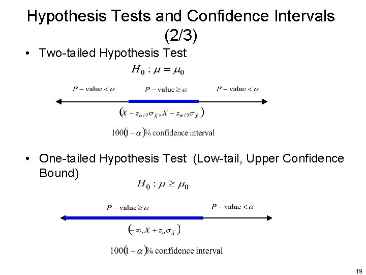
Hypothesis Tests and Confidence Intervals (2/3) • Two-tailed Hypothesis Test • One-tailed Hypothesis Test (Low-tail, Upper Confidence Bound) 19

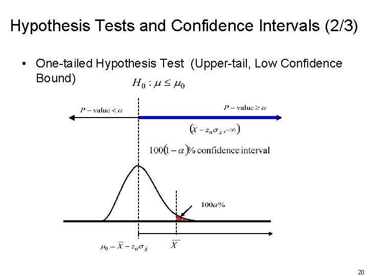
Hypothesis Tests and Confidence Intervals (2/3) • One-tailed Hypothesis Test (Upper-tail, Low Confidence Bound) 20

Tests for a Population Proportion (1/2) • A population proportion is simply a population mean for a population of 0’s and 1’s – A Bernoulli population • We have a sample that consists of successes and failures – Thus, we have hypothesis concerned with a population proportion, it is natural to base the test on the sample proportion 21

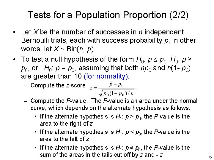
Tests for a Population Proportion (2/2) • Let X be the number of successes in n independent Bernoulli trials, each with success probability p; in other words, let X ~ Bin(n, p) • To test a null hypothesis of the form H 0: p p 0, H 0: p ≥ p 0, or H 0: p = p 0, assuming that both np 0 and n(1 - p 0) are greater than 10 (for normality): – Compute the z-score – Compute the P-value. The P-value is an area under the normal curve, which depends on the alternate hypothesis as follows: • If the alternate hypothesis is H 1: p > p 0, the P-value is the area to the right of z • If the alternate hypothesis is H 1: p < p 0, the P-value is the area to the left of z • If the alternate hypothesis is H 1: p p 0, the P-value is the sum of the areas in the tails cut off by z and - z 22

Small Sample Test for a Population Mean • When we had a large sample we used the sample standard deviation s to approximate the population deviation – When the sample size is small, s may not be close to , which invalidates this large-sample method • However, when the population is approximately normal, the Student’s t distribution can be used – The only time that we don’t use the Student’s t distribution for this situation is when the population standard deviation is known. Then we are no longer approximating and we should use the z-test 23

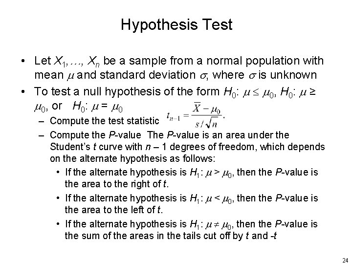
Hypothesis Test • Let X 1, …, Xn be a sample from a normal population with mean and standard deviation , where is unknown • To test a null hypothesis of the form H 0: 0, H 0: ≥ 0, or H 0: = 0 – Compute the test statistic – Compute the P-value The P-value is an area under the Student’s t curve with n – 1 degrees of freedom, which depends on the alternate hypothesis as follows: • If the alternate hypothesis is H 1: > 0, then the P-value is the area to the right of t. • If the alternate hypothesis is H 1: < 0, then the P-value is the area to the left of t. • If the alternate hypothesis is H 1: 0, then the P-value is the sum of the areas in the tails cut off by t and -t 24

Large Sample Tests for the Difference Between Two Means • Now, we are interested in determining whether or not the means of two populations are equal • The data will consist of two (independent) samples, one from each population • We will compute the difference of the sample means – Since each of the sample means follows an approximate normal distribution, the difference is approximately normal as well – If the difference is far from zero, we will conclude that the population means are different – If the difference is close to zero, we will conclude that the population means might be the same 25

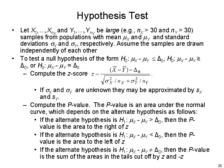
Hypothesis Test • Let X 1, …, Xn. X and Y 1, …, Yn. Y be large (e. g. , n. X > 30 and n. Y > 30) samples from populations with mean X and Y and standard deviations X and Y, respectively. Assume the samples are drawn independently of each other • To test a null hypothesis of the form H 0: X - Y Δ 0, H 0: X - Y ≥ Δ 0, or H 0: X - Y = Δ 0 – Compute the z-score • If X and Y are unknown they may be approximated by s. X and s. Y. – Compute the P-value. The P-value is an area under the normal curve, which depends on the alternate hypothesis as follows: • If the alternate hypothesis is H 1: X - Y > Δ 0, then the Pvalue is the area to the right of z • If the alternate hypothesis is H 1: X - Y < Δ 0, then the Pvalue is the area to the left of z • If the alternate hypothesis is H 1: X - Y Δ 0, then the P-value is the sum of the areas in the tails cut off by z and -z 26

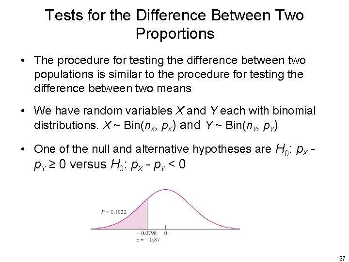
Tests for the Difference Between Two Proportions • The procedure for testing the difference between two populations is similar to the procedure for testing the difference between two means • We have random variables X and Y each with binomial distributions. X ~ Bin(n. X, p. X) and Y ~ Bin(n. Y, p. Y) • One of the null and alternative hypotheses are H 0: p. X - p. Y ≥ 0 versus H 0: p. X - p. Y < 0 27

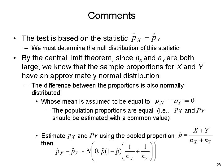
Comments • The test is based on the statistic – We must determine the null distribution of this statistic • By the central limit theorem, since n. X and n. Y are both large, we know that the sample proportions for X and Y have an approximately normal distribution – The difference between the proportions is also normally distributed • Whose mean is assumed to be equal to – The population proportions are equal (i. e. , and should be estimated with a common value) • Estimate then and using the pooled proportion 28

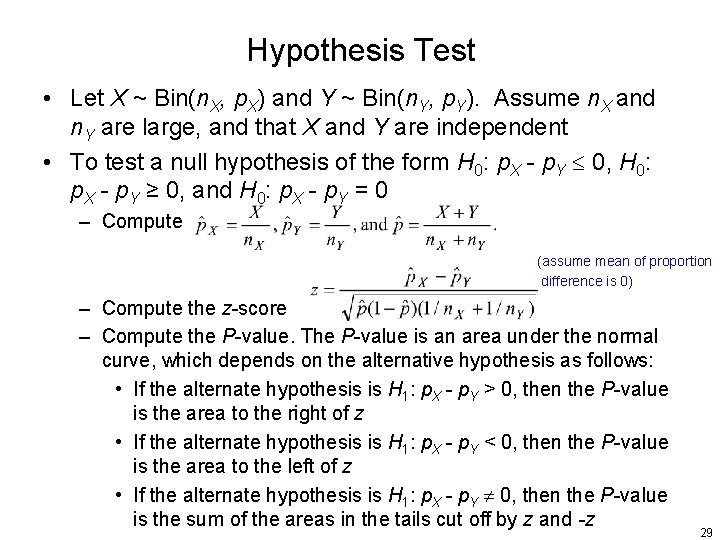
Hypothesis Test • Let X ~ Bin(n. X, p. X) and Y ~ Bin(n. Y, p. Y). Assume n. X and n. Y are large, and that X and Y are independent • To test a null hypothesis of the form H 0: p. X - p. Y 0, H 0: p. X - p. Y ≥ 0, and H 0: p. X - p. Y = 0 – Compute (assume mean of proportion difference is 0) – Compute the z-score – Compute the P-value. The P-value is an area under the normal curve, which depends on the alternative hypothesis as follows: • If the alternate hypothesis is H 1: p. X - p. Y > 0, then the P-value is the area to the right of z • If the alternate hypothesis is H 1: p. X - p. Y < 0, then the P-value is the area to the left of z • If the alternate hypothesis is H 1: p. X - p. Y 0, then the P-value is the sum of the areas in the tails cut off by z and -z 29

Small Sample Tests for the Difference Between Two Means • The t test can be used in some cases where samples are small, and thus the Central Limit Theorem does not apply • If both populations are approximately normal, the Student’s t distribution can be used to construct a hypothesis test 30

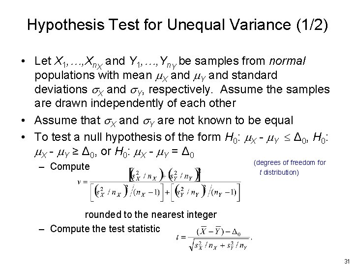
Hypothesis Test for Unequal Variance (1/2) • Let X 1, …, Xn. X and Y 1, …, Yn. Y be samples from normal populations with mean X and Y and standard deviations X and Y, respectively. Assume the samples are drawn independently of each other • Assume that X and Y are not known to be equal • To test a null hypothesis of the form H 0: X - Y Δ 0, H 0: X - Y ≥ Δ 0, or H 0: X - Y = Δ 0 – Compute (degrees of freedom for t distribution) rounded to the nearest integer – Compute the test statistic 31

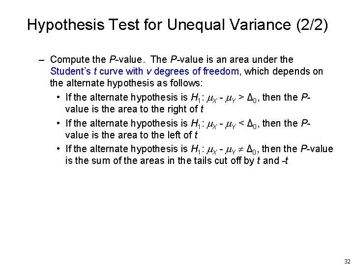
Hypothesis Test for Unequal Variance (2/2) – Compute the P-value. The P-value is an area under the Student’s t curve with v degrees of freedom, which depends on the alternate hypothesis as follows: • If the alternate hypothesis is H 1: X - Y > Δ 0, then the Pvalue is the area to the right of t • If the alternate hypothesis is H 1: X - Y < Δ 0, then the Pvalue is the area to the left of t • If the alternate hypothesis is H 1: X - Y Δ 0, then the P-value is the sum of the areas in the tails cut off by t and -t 32

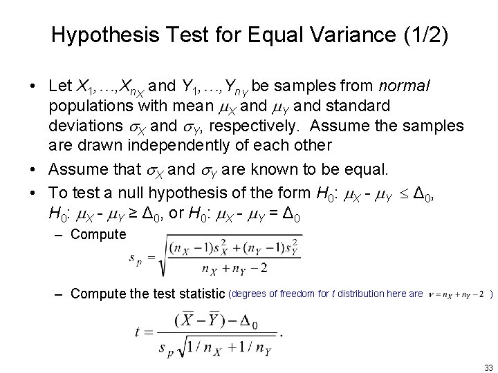
Hypothesis Test for Equal Variance (1/2) • Let X 1, …, Xn. X and Y 1, …, Yn. Y be samples from normal populations with mean X and Y and standard deviations X and Y, respectively. Assume the samples are drawn independently of each other • Assume that X and Y are known to be equal. • To test a null hypothesis of the form H 0: X - Y Δ 0, H 0: X - Y ≥ Δ 0, or H 0: X - Y = Δ 0 – Compute the test statistic (degrees of freedom for t distribution here are ) 33

Hypothesis Test for Equal Variance (2/2) – Compute the P-value. The P-value is an area under the Student’s t curve with v degrees of freedom, which depends on the alternate hypothesis as follows: • If the alternate hypothesis is H 1: X - Y > Δ 0, then the Pvalue is the area to the right of t • If the alternate hypothesis is H 1: X - Y < Δ 0, then the Pvalue is the area to the left of t • If the alternate hypothesis is H 1: X - Y Δ 0, then the P-value is the sum of the areas in the tails cut off by t and -t 34

Tests with Paired Data • Recall in in Chapter 5 that sometimes it is better to design a two-sample experiment so that each item in one sample is paired with an item in the other • Here we present a method for testing hypotheses involving the difference between two population means on the basis of such paired data • If the sample is large, the Di (i. e. , the population of differences) need not be normally distributed, the test statistic is – and a z-test should be performed 35

Hypothesis Test • Let (X 1, Y 1), …, (Xn, Yn) be sample of ordered pairs whose differences D 1, …, Dn are a sample from a normal population with mean D • To test a null hypothesis of the form H 0: D 0, H 0: D ≥ 0, or H 0: D = 0 – Compute the test statistic – Compute the P-value. The P-value is an area under the Student’s t curve with n – 1 degrees of freedom, which depends on the alternate hypothesis as follows • If the alternate hypothesis is H 1: D > 0, then the P-value is the area to the right of t • If the alternate hypothesis is H 1: D < 0, then the P-value is the area to the left of t • If the alternate hypothesis is H 1: D 0, then the P-value is the sum of the areas in the tails cut off by t and -t 36

Chi-Square (χ2) Tests • A generalization of the Bernoulli trial is the multinomial trial, which is an experiment that can result in any one of k outcomes, where k ≥ 2. – We have already discussed this in Chapter 4 • Suppose we roll a six-sided die 600 times – The results obtained are called the observed values – To test the null hypothesis that p 1= p 2= p 3= p 4= p 5= p 6= 1/6, we calculate the expected values for the given outcome – The idea behind the hypothesis test is that if H 0 is true, then the observed and expected values are likely to be close to each other 37

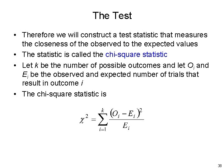
The Test • Therefore we will construct a test statistic that measures the closeness of the observed to the expected values • The statistic is called the chi-square statistic • Let k be the number of possible outcomes and let Oi and Ei be the observed and expected number of trials that result in outcome i • The chi-square statistic is 38

Decision for a Test • The larger the value of χ2, the stronger the evidence against H 0 • To determine the P-value for the test, we must know the null distribution of this test statistic • When the expected values are all sufficiently large, a good approximation is available. It is called the chisquare distribution with k – 1 degrees of freedom – Use of the chi-square distribution is appropriate whenever all the expected values are greater than or equal to 5 • A table for the chi-square distribution is provided in Appendix A, Table A. 6 39

Chi-Square (χ2) Distribution 40

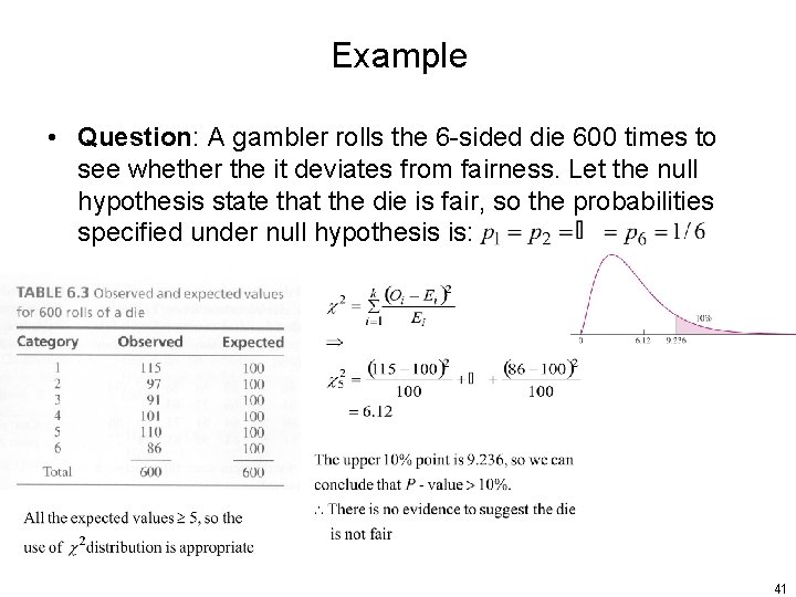
Example • Question: A gambler rolls the 6 -sided die 600 times to see whether the it deviates from fairness. Let the null hypothesis state that the die is fair, so the probabilities specified under null hypothesis is: 41

Chi-Square (χ2) Tests for Homogeneity (1/2) • Sometimes several multinomial trials (experiments) are conducted, each with the same set of possible outcomes • The null hypothesis is that the probabilities of the outcomes are the same for each experiment • There is a chi-squared statistic for testing for homogeneity • We can use a contingency table to record the observed values of different experiments • The null hypothesis the proportion of different outcomes is the same for all experiments 42

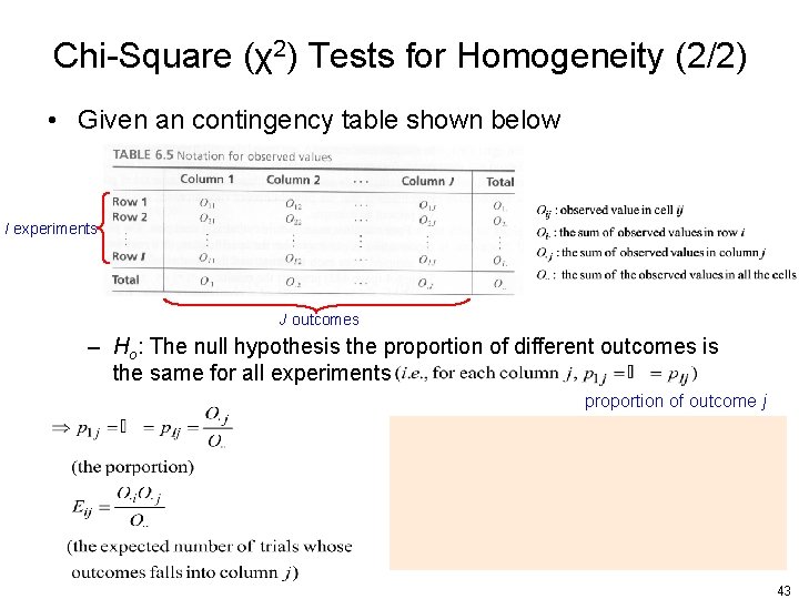
Chi-Square (χ2) Tests for Homogeneity (2/2) • Given an contingency table shown below I experiments J outcomes – Ho: The null hypothesis the proportion of different outcomes is the same for all experiments proportion of outcome j 43

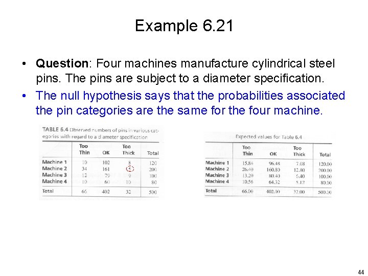
Example 6. 21 • Question: Four machines manufacture cylindrical steel pins. The pins are subject to a diameter specification. • The null hypothesis says that the probabilities associated the pin categories are the same for the four machine. 44

Chi-Square (χ2) Tests for Independence • There is also a chi-square test for independence between rows and columns in a contingency table • The null hypothesis is that the classification of the categories of one measurement do not depend on the classification of the categories of another measurement 45

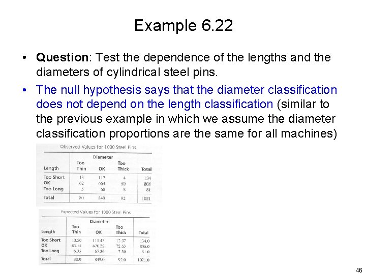
Example 6. 22 • Question: Test the dependence of the lengths and the diameters of cylindrical steel pins. • The null hypothesis says that the diameter classification does not depend on the length classification (similar to the previous example in which we assume the diameter classification proportions are the same for all machines) 46

Fixed-Level Testing • A hypothesis test measures the plausibility of the null hypothesis by producing a P-value – The smaller the P-value, the less plausible the null hypothesis • There is no scientifically valid dividing line between plausibility and implausibility, so it is impossible to specify a “correct” P-value below which we should reject H 0 – It is best simply to report the P-value instead of making a firm decision whether or not to reject • If a decision is going to be made on the basis of a hypothesis test, there is no choice but to pick a cut-off point for the P-value – When this is done, the test is referred to as a fixed-level test 47

Conducting Fixed-Level Testing • To conduct a fixed-level test: – Choose a number , where 0 < < 1. This is called the significance level, or the level, of the test – Compute the P-value in the usual way – If P , reject H 0. If P > , do not reject H 0 48

Comments on Fixed-Level Testing • In a fixed-level test, a critical point is a value of the test statistic that produces a P-value exactly equal to • A critical point is a dividing line for the test statistic just as the significance level is a dividing line for the P-value – If the test statistic is on one side of the critical point, the P-value will be less than , and H 0 will be rejected – If the test statistic is on the other side of the critical point, the Pvalue will be more than , and H 0 will not be rejected • The region on the side of the critical point that leads to rejection is called the rejection region – The critical point itself is also in the rejection region 49

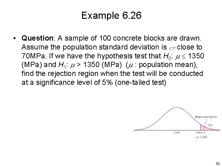
Example 6. 26 • Question: A sample of 100 concrete blocks are drawn. Assume the population standard deviation is close to 70 MPa. If we have the hypothesis test that H 0: 1350 (MPa) and H 1: > 1350 (MPa) ( : population mean), find the rejection region when the test will be conducted at a significance level of 5% (one-tailed test) 50

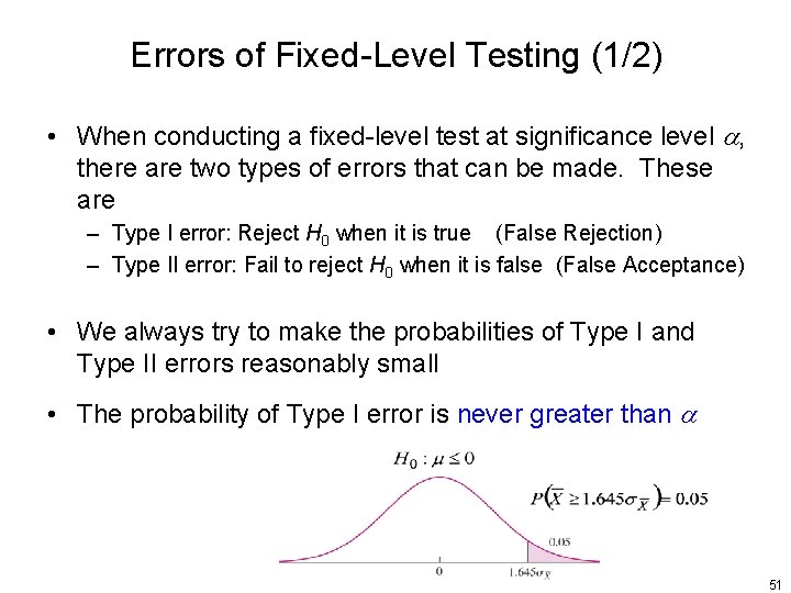
Errors of Fixed-Level Testing (1/2) • When conducting a fixed-level test at significance level , there are two types of errors that can be made. These are – Type I error: Reject H 0 when it is true (False Rejection) – Type II error: Fail to reject H 0 when it is false (False Acceptance) • We always try to make the probabilities of Type I and Type II errors reasonably small • The probability of Type I error is never greater than 51

Errors of Fixed-Level Testing (2/2) • The smaller we make the probability of a type I error, the larger the probability of type II error becomes (why? ) 52

Power • A hypothesis test results in Type II error if H 0 is not rejected when it is false • The power of the test is the probability of rejecting H 0 when it is false. Therefore, Power = 1 – P(Type II error) – To be useful, a test must have reasonable small probabilities of both type I and type II errors – The type I error is kept small by choosing a small value of as the significance level – If the power is large, then the probability of type II error is small as well, and the test is a useful one • The purpose of a power calculation is to determine whether or not a hypothesis test, when performed, is likely to reject H 0 in the event that H 0 is false 53

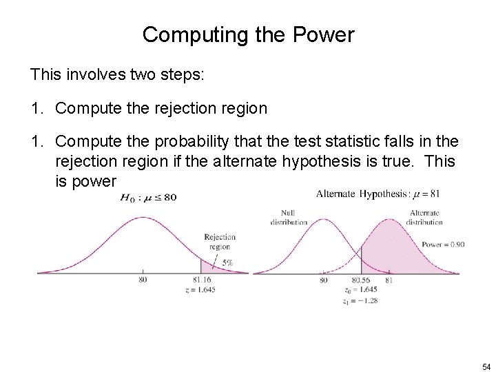
Computing the Power This involves two steps: 1. Compute the rejection region 1. Compute the probability that the test statistic falls in the rejection region if the alternate hypothesis is true. This is power 54

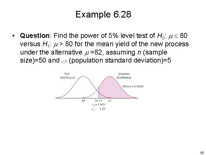
Example 6. 28 • Question: Find the power of 5% level test of H 0: 80 versus H 1: > 80 for the mean yield of the new process under the alternative =82, assuming n (sample size)=50 and (population standard deviation)=5 55

Comments on Power • The power depends on which alternate value is chosen, and can range from barely great than the significance level (when the alternate is very close to the null) all the way up to 1 (when the alternate is far from the null) • When power is not large enough, it can be increased by increasing the sample size 56

Summary • We learned about: – Large sample tests for a population mean – Drawing conclusions from the results of hypothesis tests – Tests for a population proportion and differences in two proportions – Small sample tests for a population mean – Large and small sample tests for the difference between two means – Tests with paired data – Chi-Square test – Errors (type I & II) of hypothesis testing 57