Hyperspectral Image Segmentation Mohammad Rayyan Ayoub Abuliel Agenda

Hyperspectral Image Segmentation Mohammad Rayyan Ayoub Abuliel

Agenda Segmentation using Minimum spanning forest Introduction Watershed segmentation Summarize

Introduction �The purpose of image segmentation is to partition an image into meaningful regions with respect to a particular application. �The segmentation is based on measurements taken from the image and might be greylevel, color, texture, depth or motion.

Why segmentation? Accurate segmentation of objects of interest in an image greatly facilitates further analysis of these objects. For example, it allows us to: �Count the number of objects of a certain type. �Measure geometric properties (e. g. , area, perimeter) of objects in the image. �Study properties of an individual object (intensity, texture, etc. )…

Segmentation vs classification! �Classification means to assign to each point in the image a tissue class, where the classes are agreed in advance �In fact the problems are inter-linked.

Hyperspectral image �Every pixel contains a detailed spectrum (>100 spectral bands) More information per pixel Dimensionality increases Advanced algorithms are required!

Watershed segmentation

GENERAL DEFINITION A drainage basin or watershed is an extent or an area of land where surface water from rain melting snow or ice converges to a single point at a lower elevation

Watershed transformation �One-band image on the input. �Value of each pixel = gradient value. �Image 2 D + Pixel values = Topographic relief. �Minimum = plateau of pixels from which one can only climb. �Catchment basin = set of pixels whose steepest slope paths reach M. �Watersheds = zones separating adjacent catchment basins.

Watershed �Different approaches may be employed to use the watershed principle for image segmentation. �Local minima of the gradient of the image may be chosen as markers. �Marker based watershed transformation.

Watershed for hyperspectral image

Marker-controlled watershed segmentation

Marker-controlled watershed segmentation �

Marker-controlled watershed segmentation �

Meyer's Flooding Algorithm One of the most common watershed algorithms was introduced by F. Meyer in the early 90's. 1. A set of markers, pixels where the flooding shall start, are chosen. Each is given a different label.

Meyer's Flooding Algorithm 2. The neighboring pixels of each marked area are inserted into a priority queue with a priority level corresponding to the gradient magnitude of the pixel.

Meyer's Flooding Algorithm 3. The pixel with the lowest priority level is extracted from the priority queue. If the neighbors of the extracted pixel that have already been labeled all have the same label, then the pixel is labeled with their label. All non-marked neighbors that are not yet in the priority queue are put into the priority queue.

Meyer's Flooding Algorithm 4. Redo step 3 until the priority queue is empty. The non-labeled pixels are the watershed lines.

Watershed 3 D

Marker-controlled watershed segmentation

Markers �The easiest way is to choose local min as markers but that leads to over-segmentation , it can be solved by reign merging after watershed. Oversegmentation Every local minima = 1 segment

Markers �There are many way to select marker , we will talk about method based on Pixel-wise classification(SVM classifier). �Output: classification map probability map

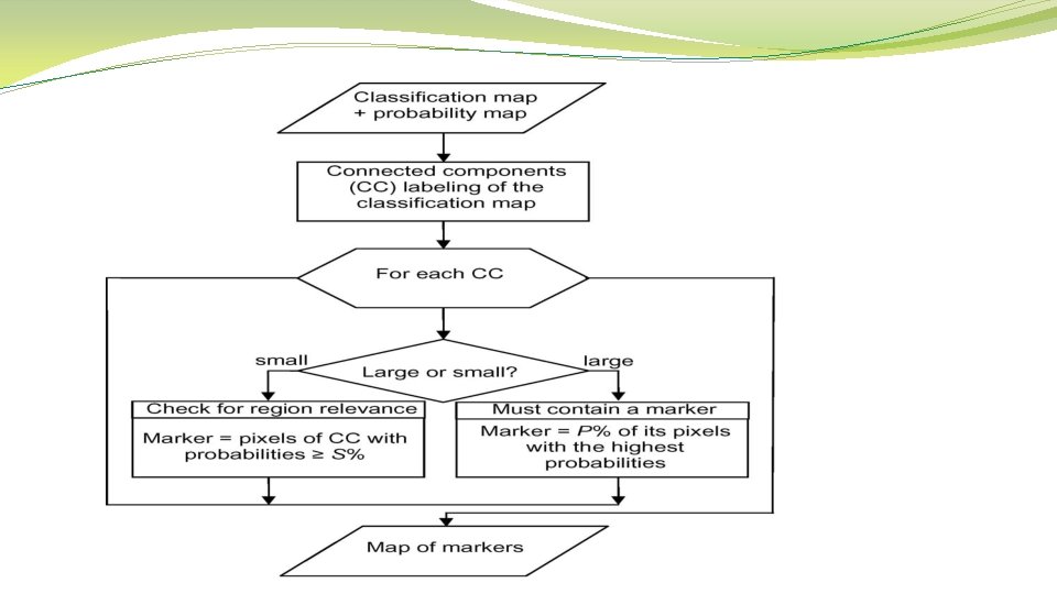
Selection of the most reliable classified pixels 1. Perform connected components labeling of the classification map. 2. Analyze each connected component: Ø If it is large (> 20 pixels) then use P% (5%) of its pixels with the highest probabilities as a marker. Ø If it is small then its pixels with probabilities > T% (90%) are used as a marker.

Selection of the most reliable classified pixels �Each connected component -> 1 or 0 marker (2250 regions -> 107 markers). �Marker is not necessarily a connected set of pixels. �Each marker has a class label classification map Map of 107 markers probability map

Gradient

Image Gradient �An image gradient is a directional change in the intensity or color in an image. � A gradient image is a scalar function Original image gradient image in the x direction gradient image in the y direction

Image Representation �hyperspectral image: �Where:

Image Gradient �To define a gradient four approaches are considered: 1. a morphological gradient on one channel. 2. a metric-based gradient on all channels. 3. a gradient defined as the supremum of morphological gradients on each channel 4. a gradient defined as the sum of morphological gradients on each channel

Morphological Gradient �The morphological gradient is a marginal gradient, it can only be applied on scalar images. �defined as the difference between channel dilation and erosion with a structuring element Bx which is the neighborhood of a point x ∈ E:

gradient supremum �The gradient supremum of morphological gradients on each channel is a vectorial gradient defined as: �Each morphological gradient must be normalized between [0; 1] before taking the supremum.

gradient weighted sum �The gradient weighted sum of morphological gradients is given by:

metric-based gradient �The metric-based gradient is a vectorial gradient defined as the difference between the supremum and the infimum of a defined distance on a unit neighbourhood B(x): �Various metric distances are available for this gradient such as: Euclidean distance, Mahalanobis distance, chi-squared distance…

MSF Segmentation

What the problem ? The purpose of image segmentation is to partition an image into meaningful regions with respect to a particular application.

Terms and structures �MST : Minimum spanning tree Given a graph G = (V, E, W), the minimum spanning tree is defined as a spanning tree T∗ = (V, ET∗ ) of G such that the sum of the edge weights of T∗ is minimal where ST is a set of all spanning trees of G.

Terms and structures �MSF : Minimum Spanning Forest Given a graph G = (V, E, W), the MSF rooted on a set of m distinct vertices {t 1, . . . , tm} consists in finding a spanning forest F∗ = (V, EF∗ ) of G, such that each distinct tree of F∗ is grown from one root ti, and the sum of the edge weights of F∗ is minimal where SF is a set of all spanning forests of G rooted on {t 1, . . . , tm}.

Terms and structures

Terms and structures �Oversegmentation : one region is detected as several ones of the image. �undersegmentation : several regions are detected as one

What the method ? �The method is based on the construction of an MSF, rooted on the markers selected by using pixelwise classification results.

The 4 steps: A. Pixelwise classification B. Selection of the most Reliable classified Pixels C. Construction of an MSF D. Majority Voting Within Connected Components

Pairwise classification The first step consists in performing a probabilistic pixelwise classification of the hyperspectral image. We propose to use a Support vector machine (SVM) classifier

The outputs of this step are the following: � 1) classification map, containing class labels for each pixel; � 2) probability map, containing probability estimates for each pixel to belong to the assigned class.

The aim: to estimate, for each pixel x, the probabilities to belong to each class of interest p = {pk = p (y = k|x), k = 1, . . . , K}. K : one of the segments. We must to give for each pixel vector P that is values Probabilities to be belonging to segment k.

Pairwise classification For this purpose, first, pairwise class probabilities rij ≈ p(y = i|y = i or j, x) are estimated using an improved implementation

Pairwise classification where A and B are estimated by minimizing the negative loglikelihood function using known training data and decision values ˆ f. Furthermore, the probabilities in (1) are computed by solving the following optimization problem:

We have a matrix for rij and we must to select the minimum line that deducted the equation : j i

Pairwise classification This problem has a unique solution and can be solved by a simple linear system. Finally, a probability map is constructed by assigning to each pixel the maximum probability estimate max(pk), k = 1, . . . , K.

B. Selection of the Most Reliable Classified Pixels The aim of this step is to choose the most reliable classified pixels in order to define suitable markers.

B. Selection of the Most Reliable Classified Pixels A simple way of marker selection consists in thresholding the probability map. In other words, if the probability of the considered pixel belonging to the assigned class k is higher than a given threshold, this pixel is selected to join the markers.

B. Selection of the Most Reliable Classified Pixels The marker pixels form connected components in the map of markers so that each connected component represents one marker.

Advantage and disadvantage Advantage : simplicity Disadvantage : 1) Each marker leads to one region in the segmentation map. Therefore, we need as many markers as the desired number of regions.

disadvantage 2) if classes ki and kj are spectrally similar, pixels belonging to one of those classes have a quasi-equal probability to belong to each of them. we risk to lose the regions corresponding to either class ki or kj in the final segmentation map. This leads to undersegmentation, which is highly undesired.

solution To mitigate this problem, we propose the following method of marker selection 1) Perform a connected-component labeling of the pixelwise classification map. For this purpose, a classical connected component algorithm using the union-find data structure.

solution 2) Analyze each connected region as follows. • If a region is large enough, it should contain a marker, which is determined as P% of the pixels within the connected component with the highest probability estimates. • If a region is small, it should lead to a marker only if it is very reliable; a potential marker is formed by pixels with probability estimates higher than a defined threshold.

each connected spatial region from the classification map is analyzed if it corresponds most probably to the spatial structure or if it is rather a classification noise

If the size of the component is large enough to consider it as a relevant region, the most reliable pixels within this region are selected as its marker. If a component contains only a few pixels, it is investigated if these pixels were classified to a particular class with a high probability. If this is the case, the considered connected component represents a small spatial structure. Thus, a marker associated with this region should be defined. Otherwise, the component is the consequence of classification noise, and we tend to eliminate it.

parameters 1) A parameter M defining if a region is considered as being large or small. 2) A parameter P, defining the percentage of pixels within the large region to be used as markers 3) The last parameter S, which is a threshold of probability estimates defining potential markers for a small region, depends on the probability of the presence of small structures in the image

C. Construction of an MSF : minimum spanning forst. The previous two steps result in a map of markers defining regions of interest in the image. The next step consists in the grouping of all the image pixels into an MSF , where each tree is rooted on a classificationderived marker.

C. Construction of an MSF each pixel is considered as a vertex v ∈ V of an undirected graph G = (V, E, W), where V and E are the sets of vertices and edges, respectively, and W is a mapping of the set of edges E into R+. Each edge ei, j ∈ E of this graph connects a couple of vertices i and j corresponding to the neighboring pixels. a weight wi, j is assigned to each edge ei, j , which indicates the degree of dissimilarity between two pixels connected by this edge. Different dissimilarity measures can be used for computing weights of edges, such as vector norms, Spectral Angle Mapper (SAM), and spectral information divergence (SID)

Different dissimilarity measure The L 1 vector norm between two pixel vectors xi = (xi 1, . . . , xi. B)T and xj = (xj 1, . . . , xj. B)T is given as

Different dissimilarity measure The SAM distance between xi and xj determines the spectral similarity between two vectors by computing the angle between them. It is defined as

Different dissimilarity measure The SID measure computes the discrepancy of probabilistic behaviors between the spectral signatures of two pixels. It is defined as Where:

Algorithm 1 Prim’s Algorithm Require: Connected graph G = (V, E, W) Ensure: Tree T∗ = (V ∗, E∗, W∗) V ∗ = {v}, v is an arbitrary vertex from V While V ∗ not = V do Choose edge ei, j ∈ E with minimal weight such that i ∈ V ∗ and j not belong to. V ∗ = V ∗ ∪ {j} E∗ = E∗ ∪ {ei, j} end while

t 1 0 r 0 0 0 1 0 8 1 2 5 14 8 5 4 0 11 15 9 0 12 14 10 0 t 2 0 16 0 12 3 11 8 0 0 5 2

t 1 0 r 0 0 2 5 0 8 1 1 5 0 t 2 0 14 8 0 0 0 12 3 0 0 5 2

t 1 0 r 0 0 8 1 1 2 5 0 t 2 0 14 5 0 4 1 10 0 16 0 12 0 0 3 5 2

t 1 0 r 0 0 8 1 1 0 t 2 0 2 5 15 5 0 4 1 10 0 2 12 0 0 3 5 2

t 1 0 r 0 0 8 1 1 0 t 2 0 2 15 1 14 4 1 0 10 12 11 0 2 0 3 5 2

t 1 0 r 0 0 1 1 0 8 t 2 0 2 15 1 4 2 0 10 14 0 1 3 8 2 5 2

t 1 0 r 0 0 1 1 0 8 t 2 0 2 15 1 4 1 2 0 3 2 8 2 5 2

t 1 0 r 0 0 1 1 0 8 t 2 1 4 1 2 0 3 2 8 2 5 2

D. Majority Voting Within Connected Components Although the most reliable classified pixels are selected as markers, it may happen that a marker is classified to the wrong class. In this case, all the pixels within the region grown from this marker risk to be wrongly classified.

D. Majority Voting Within Connected Components we propose to postprocess the classification map by applying a simple majority voting technique which has shown good performances for spectralspatial classification. For this purpose, connected-component labeling is applied on the obtained spectral-spatial classification map. Furthermore, for every connected component (region), all the pixels are assigned to the most frequent class when analyzing a pixelwise classification map within this region.

Experiment �Classification of the Indiana Image (A three-band false color image)

Experiment Method: �- Pixelwise classification �- connected component 1) If it contained more than M = 20 pixels, P = 5% of its pixels with the highest probability estimates were selected as a marker for this component. 2) Otherwise, if a connected component contained pixels with the corresponding probability estimates not lower than the threshold S, these pixels were used as a marker.

. Indiana image. (a)Three-band color composite (837, 636, and 537 nm). (b)Reference data: . (c) Pixelwise classification map. (d) Probability map (probability estimates for each pixel to belong to the assigned class). (e) Scale of colors to represent the probability estimates in a probability map, from 0% probability at the bottom to 100% probability at the top. (f) Classification map obtained by the proposed scheme, using the SAM dissimilarity measure and including a majority voting step.

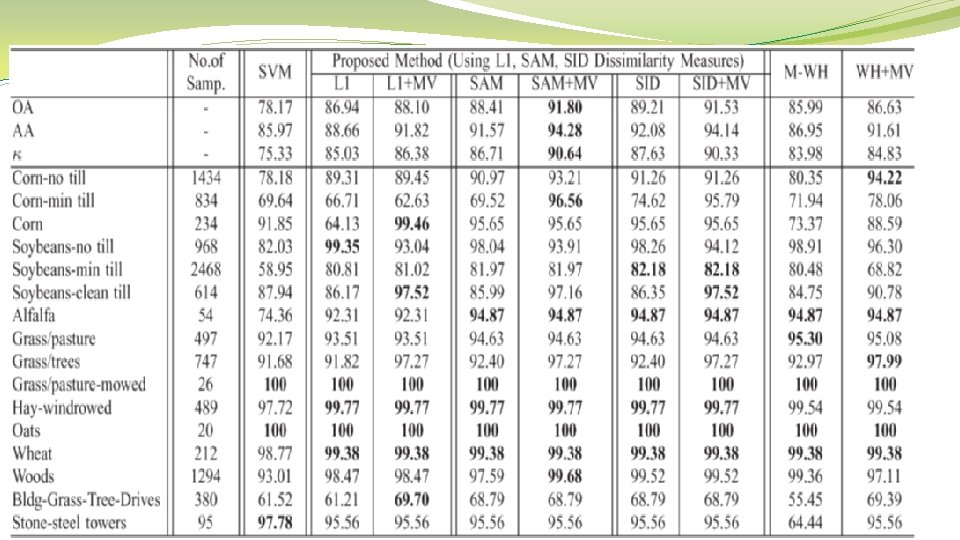
Experimental results � 1) almost no oversegmentation is present in the obtained segmentation map (since one marker led to one region, a segmentation map contains 107 regions ). � 2) The majority voting step additionally improves most of the accuracies � 3) The best global accuracies are achieved by the proposed method when using the SAM dissimilarity measure and including a majority voting step

comparion Watershed MSF Not efficient speed Accepted speed In many cases the image my oversegment Almost no oversegmentation Segment borders not accurate

Summarize �A large number of spectral channels in a hyperspectral image increase the potential of discriminating physical materials and structures in a scene. �It presents challenges to image analysis because of the huge volume of data that the hyperspectral image usually consists of. �Segmentation can be used as a way to add spatial information to spectral based classification like pixelwise classification. �There are many way to get segmentation and regular algorithm must be adapt to work with HS. �Segmentation is important process for image analysis.

Questions

references �Segmentation and Classification of Hyperspectral Images Using Minimum Spanning Forest Grown From Automatically Selected Markers Yuliya Tarabalka, Jocelyn Chanussot, and Jón Atli Benediktsson IEEE Transactions on System Man and Cybernetics, Vol 40(5), 2010 �Object Segmentation in Hyperspectral Images Susi Huaman De la Vega, Dr. Vidya Manian �SEGMENTATION AND CLASSIFICATION OF HYPERSPECTRAL DATA USING WATERSHED Yuliya Tarabalka 1, 2, Jocelyn Chanussot 1, Jon Atli Benediktsson 2, Jesus Angulo 3, and Mathieu Fauvel 1, 2

references �A new spatio-spectral morphological segmentation for multispectral remote sensing images G. NOYELy & J. ANGULOy and D. JEULINy