Hybridisation Solver Cooperation in ECLi PSe Introduction Motivation

Hybridisation Solver Cooperation in ECLi. PSe

Introduction ¡ ¡ Motivation Sending Constraints to Different Solvers Probing Column Generation 2

Why Use Multiple Solvers? ¡ Real problems comprise different subproblems Different solvers/algorithms suit different subproblems ¡ Global reasoning can be achieved in different ways Linear solvers reason globally on linear constraints Domain solvers support application-specific global constraints ¡ Solvers complement each other Optimisation versus feasibility New and adapted forms of cooperation (e. g. Linear relaxation as a heuristic) ¡ Growing experience IC-Parc, CMU, Bologna, Bouygues, ILOG…see CPAIOR 3

How to Use Multiple Solvers ¡ Problem Decomposition Send subproblem constraints to subproblem solver e. g. Continuous/discrete circuits; Process scheduling ¡ Redundant Solving Send a constraint to more than one solver e. g. Hoist scheduling; Progressive Party Problem 4

Hybridising ic and eplex ¡ Local propagation ·e. g. interval propagation ·more general constraints ·handle integers directly ·Favourable example: Variable Bounds: [X 1, …, X 100] : : 1. . 100 ¡ Global algorithmic solving ·e. g. Simplex, Gauss ·restricted class of constraints ·finds optimum without search ·Favourable example: Variable Bounds: [X 1, X 2] : : 1. . 100 Previous Constraints: X 1 < X 2 , … , X 98 < X 99 Resulting Bounds: X 1 : : 1. . 2, …, X 99 : : 99. . 100 New Constraint: X 1 >= 3 Result (1 step): failure! New Constraints: X 1 > X 2, X 2 > X 1 Result (1 step): failure! 5

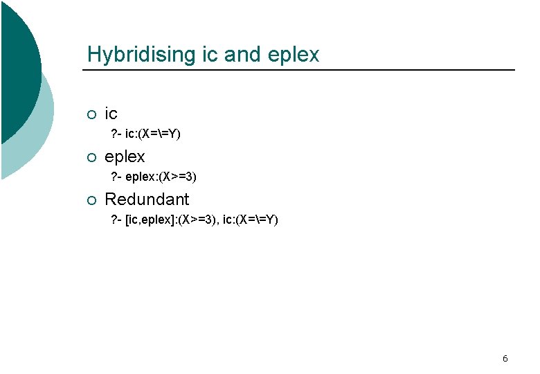
Hybridising ic and eplex ¡ ic ? - ic: (X==Y) ¡ eplex ? - eplex: (X>=3) ¡ Redundant ? - [ic, eplex]: (X>=3), ic: (X==Y) 6

Techniques ¡ ¡ Shared Variables Linear constraints to ic and eplex Reduced cost propagation Other methods (Milano tutorial) 7

Introduction ¡ ¡ Motivation Sending Constraints to Different Solvers Probing Column Generation 8

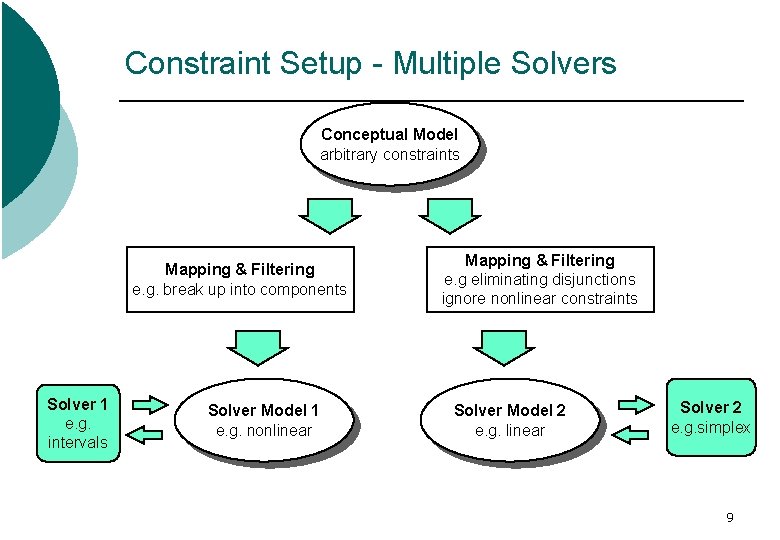
Constraint Setup - Multiple Solvers Conceptual Model arbitrary constraints Mapping & Filtering e. g. break up into components Solver 1 e. g. intervals Solver Model 1 e. g. nonlinear Mapping & Filtering e. g eliminating disjunctions ignore nonlinear constraints Solver Model 2 e. g. linear Solver 2 e. g. simplex 9

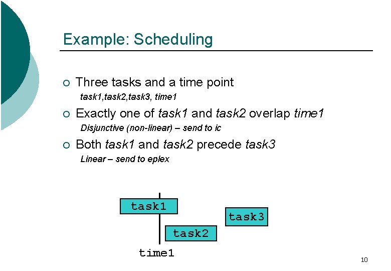
Example: Scheduling ¡ Three tasks and a time point task 1, task 2, task 3, time 1 ¡ Exactly one of task 1 and task 2 overlap time 1 Disjunctive (non-linear) – send to ic ¡ Both task 1 and task 2 precede task 3 Linear – send to eplex task 1 task 3 task 2 time 1 10

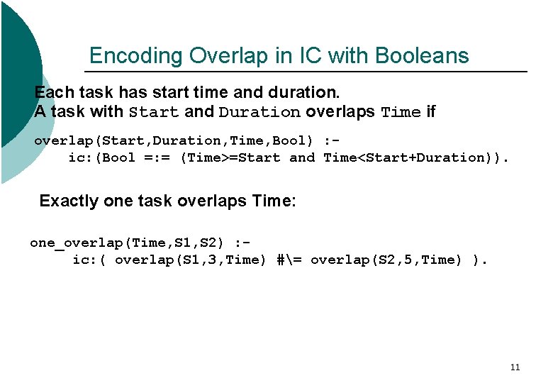
Encoding Overlap in IC with Booleans Each task has start time and duration. A task with Start and Duration overlaps Time if overlap(Start, Duration, Time, Bool) : ic: (Bool =: = (Time>=Start and Time<Start+Duration)). Exactly one task overlaps Time: one_overlap(Time, S 1, S 2) : ic: ( overlap(S 1, 3, Time) #= overlap(S 2, 5, Time) ). 11

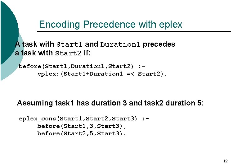
Encoding Precedence with eplex A task with Start 1 and Duration 1 precedes a task with Start 2 if: before(Start 1, Duration 1, Start 2) : eplex: (Start 1+Duration 1 =< Start 2). Assuming task 1 has duration 3 and task 2 duration 5: eplex_cons(Start 1, Start 2, Start 3) : before(Start 1, 3, Start 3), before(Start 2, 5, Start 3). 12

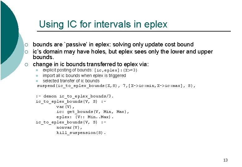
Using IC for intervals in eplex ¡ ¡ ¡ bounds are `passive’ in eplex: solving only update cost bound ic’s domain may have holes, but eplex sees only the lower and upper bounds. change in ic bounds transferred to eplex via: explicit posting of bounds: [ic, eplex]: (X>=3) l import all ic bounds when eplex is triggered l selected transfer of ic bounds suspend(ic_to_eplex_bounds(X, S), 7, [X->ic: min, X->ic: max], S), l : - demon ic_to_eplex_bounds/3. ic_to_eplex_bounds(V, S) : var(V), ic: get_bounds(V, Min, Max), eplex: (V: : Min. . Max). ic_to_eplex_bounds(V, S) : nonvar(V), kill_suspension(S). 13

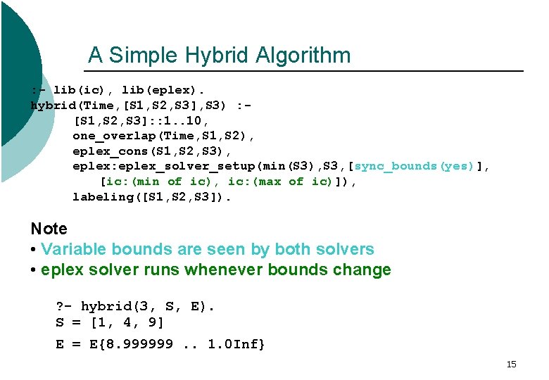
A Simple Hybrid Algorithm : - lib(ic), lib(eplex). hybrid(Time, [S 1, S 2, S 3], S 3) : [S 1, S 2, S 3]: : 1. . 10, one_overlap(Time, S 1, S 2), eplex_cons(S 1, S 2, S 3), eplex: eplex_solver_setup(min(S 3), S 3, [sync_bounds(yes)], [ic: (min of ic), ic: (max of ic)]), labeling([S 1, S 2, S 3]). Note • Variable bounds are seen by both solvers • eplex solver runs whenever bounds change ? - hybrid(3, S, E). S = [1, 4, 9] E = E{8. 999999. . 1. 0 Inf} 15

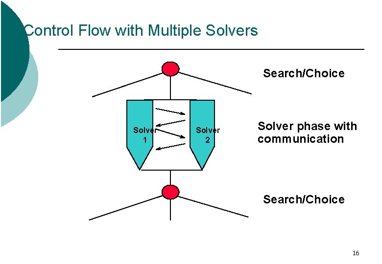
Control Flow with Multiple Solvers Search/Choice Solver 1 Solver 2 Solver phase with communication Search/Choice 16

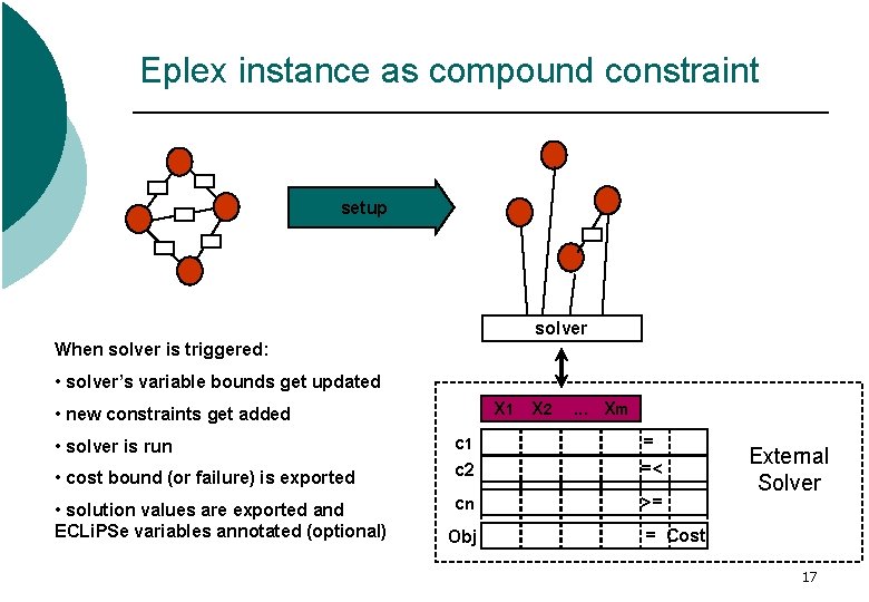
Eplex instance as compound constraint setup solver When solver is triggered: • solver’s variable bounds get updated X 1 X 2 • new constraints get added • solver is run • cost bound (or failure) is exported • solution values are exported and ECLi. PSe variables annotated (optional) . . . Xm c 1 c 2 = =< cn >= Obj External Solver = Cost 17

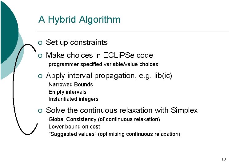
A Hybrid Algorithm ¡ Set up constraints ¡ Make choices in ECLi. PSe code programmer specified variable/value choices ¡ Apply interval propagation, e. g. lib(ic) Narrowed Bounds Empty intervals Instantiated integers ¡ Solve the continuous relaxation with Simplex Global Consistency (of continuous relaxation) Lower bound on cost “Suggested values” (optimising continuous relaxation) 18

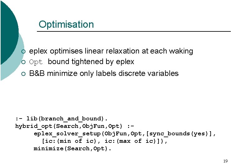
Optimisation ¡ eplex optimises linear relaxation at each waking Opt bound tightened by eplex ¡ B&B minimize only labels discrete variables ¡ : - lib(branch_and_bound). hybrid_opt(Search, Obj. Fun, Opt) : eplex_solver_setup(Obj. Fun, Opt, [sync_bounds(yes)], [ic: (min of ic), ic: (max of ic)]), minimize(Search, Opt). 19

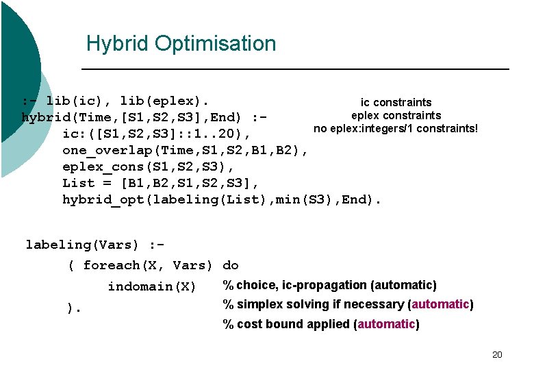
Hybrid Optimisation : - lib(ic), lib(eplex). ic constraints eplex constraints hybrid(Time, [S 1, S 2, S 3], End) : no eplex: integers/1 constraints! ic: ([S 1, S 2, S 3]: : 1. . 20), one_overlap(Time, S 1, S 2, B 1, B 2), eplex_cons(S 1, S 2, S 3), List = [B 1, B 2, S 1, S 2, S 3], hybrid_opt(labeling(List), min(S 3), End). labeling(Vars) : ( foreach(X, Vars) do indomain(X) ). % choice, ic-propagation (automatic) % simplex solving if necessary (automatic) % cost bound applied (automatic) 20

Introduction ¡ ¡ ¡ Motivation Sending Constraints to Different Solvers Linearising Logical Constraints Probing Column Generation 36

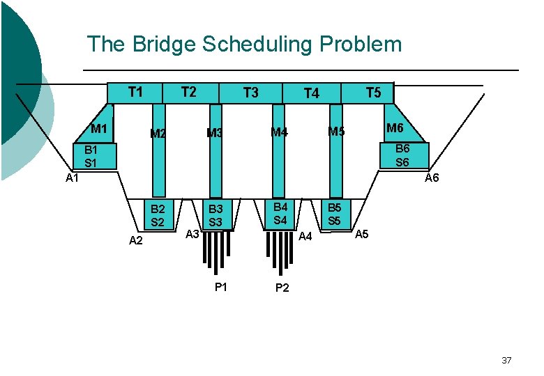
The Bridge Scheduling Problem T 1 M 1 T 2 T 3 M 2 T 5 T 4 M 6 M 5 M 4 B 6 S 6 B 1 S 1 A 6 B 2 S 2 A 3 B 3 S 3 B 4 S 4 B 5 S 5 A 4 P 1 A 5 P 2 37

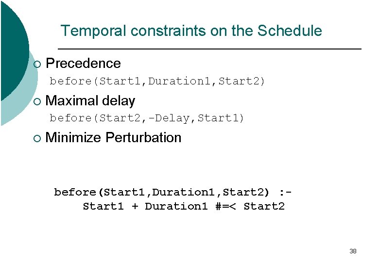
Temporal constraints on the Schedule ¡ Precedence before(Start 1, Duration 1, Start 2) ¡ Maximal delay before(Start 2, -Delay, Start 1) ¡ Minimize Perturbation before(Start 1, Duration 1, Start 2) : Start 1 + Duration 1 #=< Start 2 38

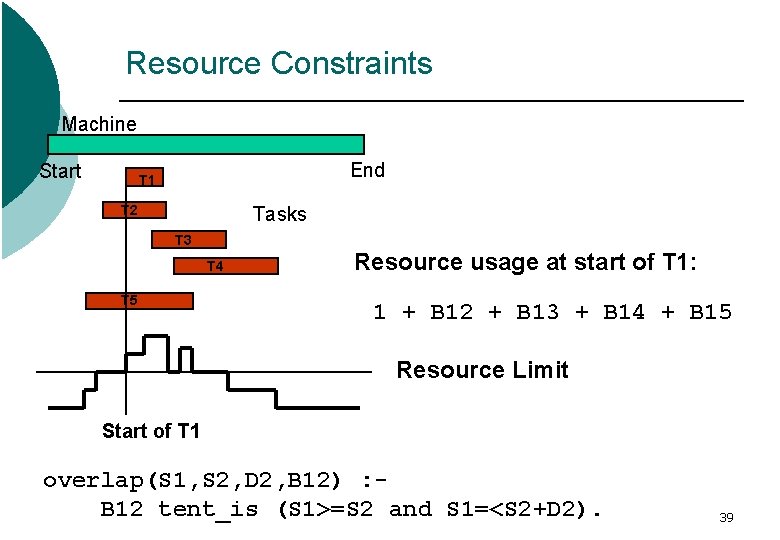
Resource Constraints Machine Start End T 1 T 2 Tasks T 3 T 4 T 5 Resource usage at start of T 1: 1 + B 12 + B 13 + B 14 + B 15 Resource Limit Start of T 1 overlap(S 1, S 2, D 2, B 12) : B 12 tent_is (S 1>=S 2 and S 1=<S 2+D 2). 39

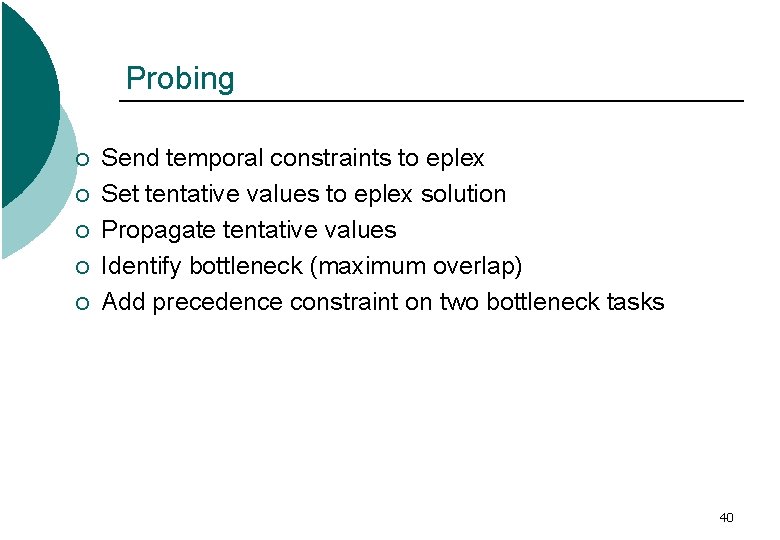
Probing ¡ ¡ ¡ Send temporal constraints to eplex Set tentative values to eplex solution Propagate tentative values Identify bottleneck (maximum overlap) Add precedence constraint on two bottleneck tasks 40

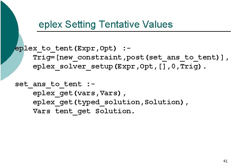
eplex Setting Tentative Values eplex_to_tent(Expr, Opt) : Trig=[new_constraint, post(set_ans_to_tent)], eplex_solver_setup(Expr, Opt, [], 0, Trig). set_ans_to_tent : eplex_get(vars, Vars), eplex_get(typed_solution, Solution), Vars tent_get Solution. 41

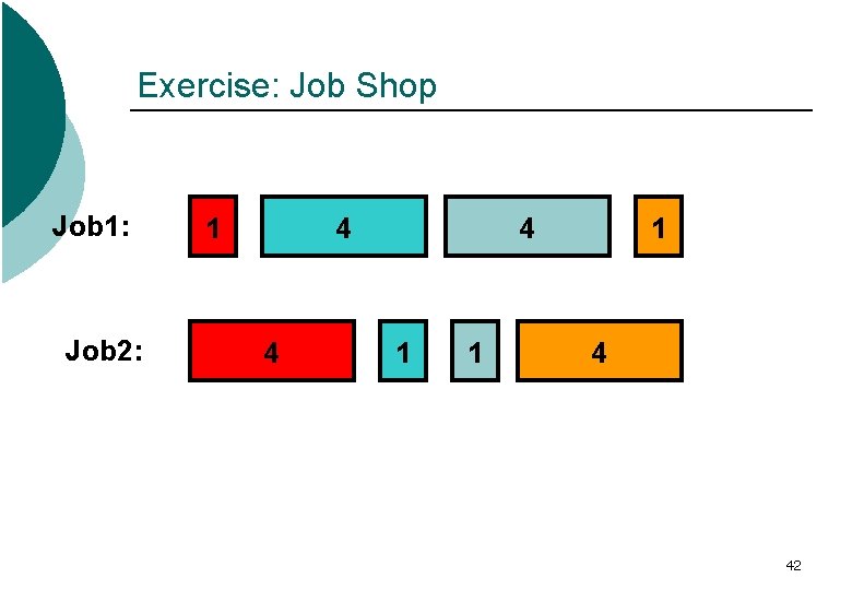
Exercise: Job Shop Job 1: Job 2: 1 4 4 4 1 1 1 4 42

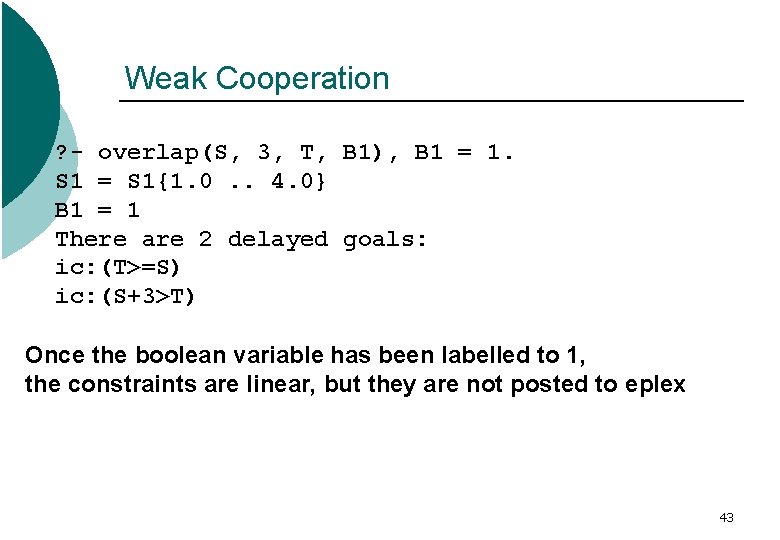
Weak Cooperation ? - overlap(S, 3, T, B 1), B 1 = 1. S 1 = S 1{1. 0. . 4. 0} B 1 = 1 There are 2 delayed goals: ic: (T>=S) ic: (S+3>T) Once the boolean variable has been labelled to 1, the constraints are linear, but they are not posted to eplex 43

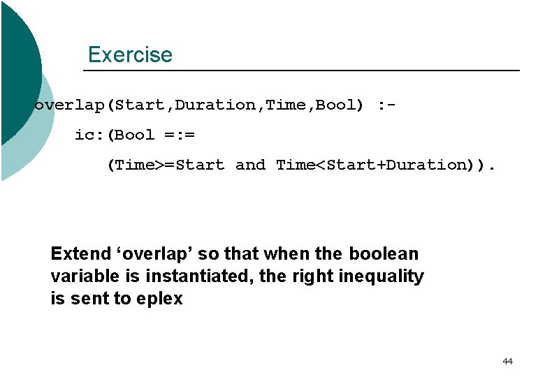
Exercise overlap(Start, Duration, Time, Bool) : ic: (Bool =: = (Time>=Start and Time<Start+Duration)). Extend ‘overlap’ so that when the boolean variable is instantiated, the right inequality is sent to eplex 44

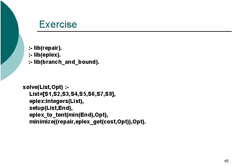
Exercise : - lib(repair). : - lib(eplex). : - lib(branch_and_bound). solve(List, Opt) : List=[S 1, S 2, S 3, S 4, S 5, S 6, S 7, S 8], eplex: integers(List), setup(List, End), eplex_to_tent(min(End), Opt), minimize((repair, eplex_get(cost, Opt)), Opt). 45

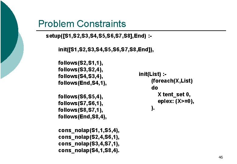
Problem Constraints setup([S 1, S 2, S 3, S 4, S 5, S 6, S 7, S 8], End) : init([S 1, S 2, S 3, S 4, S 5, S 6, S 7, S 8, End]), follows(S 2, S 1, 1), follows(S 3, S 2, 4), follows(S 4, S 3, 4), follows(End, S 4, 1), follows(S 6, S 5, 4), follows(S 7, S 6, 1), follows(S 8, S 7, 1), follows(End, S 8, 4), init(List) : (foreach(X, List) do X tent_set 0, eplex: (X>=0), ). cons_nolap(S 1, 1, S 5, 4), cons_nolap(S 2, 4, S 6, 1), cons_nolap(S 3, 4, S 7, 1), cons_nolap(S 4, 1, S 8, 4). 46

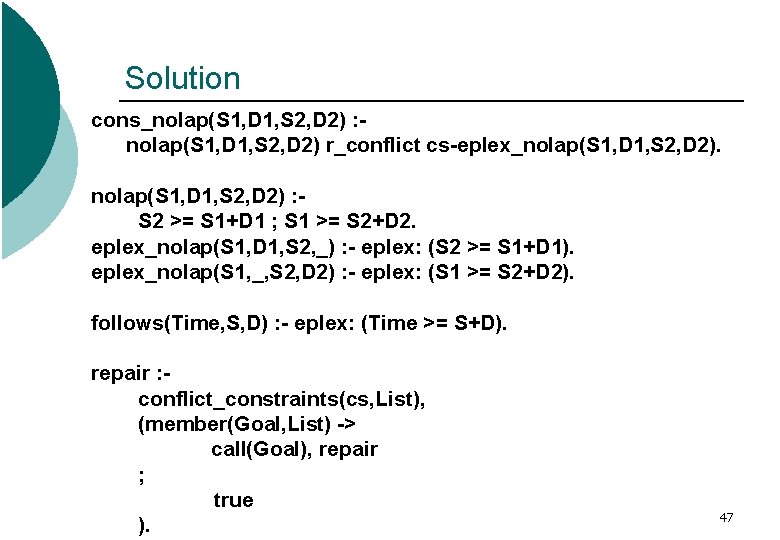
Solution cons_nolap(S 1, D 1, S 2, D 2) : nolap(S 1, D 1, S 2, D 2) r_conflict cs-eplex_nolap(S 1, D 1, S 2, D 2) : S 2 >= S 1+D 1 ; S 1 >= S 2+D 2. eplex_nolap(S 1, D 1, S 2, _) : - eplex: (S 2 >= S 1+D 1). eplex_nolap(S 1, _, S 2, D 2) : - eplex: (S 1 >= S 2+D 2). follows(Time, S, D) : - eplex: (Time >= S+D). repair : conflict_constraints(cs, List), (member(Goal, List) -> call(Goal), repair ; true ). 47

Introduction ¡ ¡ ¡ Motivation Sending Constraints to Different Solvers Linearising Logical Constraints Probing Column Generation 48

Objectives ¡ Devise Hybrid techniques ¡ Encapsulate Mystifying techniques ¡ Apply To practical problems in IP and transport 49

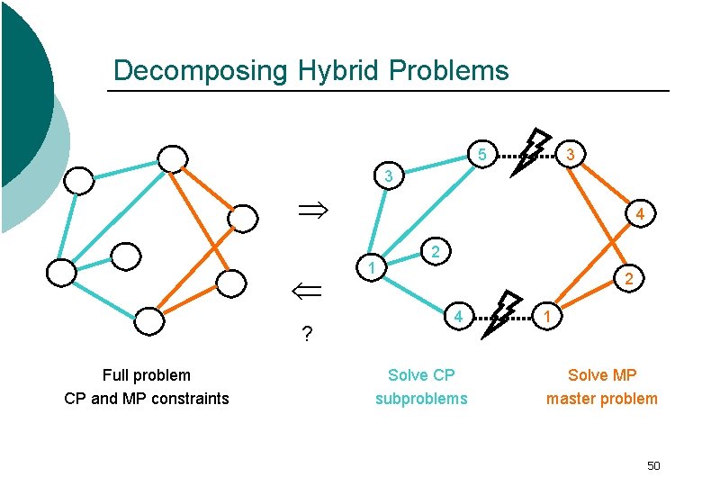
Decomposing Hybrid Problems 5 3 3 ? Full problem CP and MP constraints 4 1 2 2 4 Solve CP subproblems 1 Solve MP master problem 50

Hybrids between CP and MP ¡ CP hybrids Flat structure MP solver as global CP constraint Exclude infeasible values from variable domains ¡ MP hybrids Hierarchical structure MP solver for master problem CP solver for subproblems Pass information inferred from optimal solutions 51

Encapsulation ¡ User identifies subproblems Separate solvers associated with master and subproblems Communication of solution information between solvers handled automatically Iteration and stopping criteria handled automatically ¡ Available as an ECLi. PSe Library 52

Applications ¡ Minimal Perturbation Scheduling Application to airline scheduling ¡ Patrol Assignment Application to emergency services ¡ Backup Route Generation Application to current internet technology ¡ Primary and Secondary Path Assignment Application to next generation internet technology 53

Column Generation (1) ¡ ¡ ¡ We can instead decompose a problem into a Master Problem and Subproblems The Subproblems find solutions to subsets of the constraints The Master Problem finds an optimum combination of those solutions (termed “columns”) 54

Example: The Multiple Vehicle Routing Problem ¡ Subproblem. V Create a “good” tour for vehicle V ¡ Master Problem Select an optimal set of tours that cover the required locations 55

Column Generation for MVRP ¡ ¡ Subproblem can be solved by any appropriate technique e. g. we use ic for MVRP subproblems The subproblem solver is independent of column generation - only a cost vector is needed for the interface 56

Column Generation - Details ¡ ¡ Choice of initial column set impacts performance Column management can become an issue For integer problems we must perform column generation within each node of a branch-and-bound tree Branching alters the subproblems 57

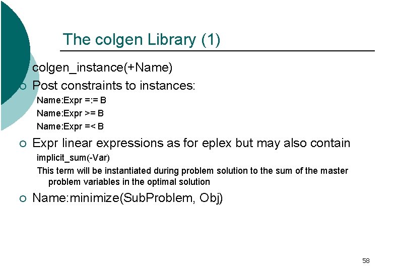
The colgen Library (1) ¡ ¡ colgen_instance(+Name) Post constraints to instances: Name: Expr =: = B Name: Expr >= B Name: Expr =< B ¡ Expr linear expressions as for eplex but may also contain implicit_sum(-Var) This term will be instantiated during problem solution to the sum of the master problem variables in the optimal solution ¡ Name: minimize(Sub. Problem, Obj) 58

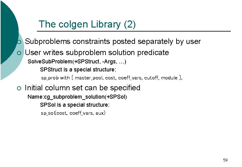
The colgen Library (2) ¡ ¡ Subproblems constraints posted separately by user User writes subproblem solution predicate Solve. Sub. Problem(+SPStruct, -Args, …) SPStruct is a special structure: sp_prob with [ master_pool, cost, coeff_vars, cutoff, module ], ¡ Initial column set can be specified Name: cg_subproblem_solution(+SPSol) SPSol is a special structure: sp_sol(cost, coeff_vars, aux) 59

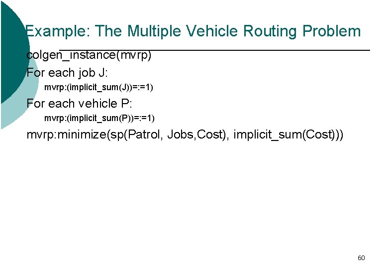
Example: The Multiple Vehicle Routing Problem colgen_instance(mvrp) For each job J: mvrp: (implicit_sum(J))=: =1) For each vehicle P: mvrp: (implicit_sum(P))=: =1) mvrp: minimize(sp(Patrol, Jobs, Cost), implicit_sum(Cost))) 60

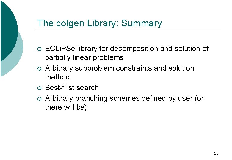
The colgen Library: Summary ¡ ¡ ECLi. PSe library for decomposition and solution of partially linear problems Arbitrary subproblem constraints and solution method Best-first search Arbitrary branching schemes defined by user (or there will be) 61

See Also ¡ ¡ CPAIOR School proceedings Milano Tutorial Le Pape / Wallace Tutorial CP Proceedings Column Generation Benders Decomposition 62