Hybrid VariationalEnsemble Data Assimilation at NCEP Daryl Kleist

Hybrid Variational-Ensemble Data Assimilation at NCEP Daryl Kleist NOAA/NWS/NCEP/EMC with acknowledgements to Kayo Ide, Dave Parrish, Jeff Whitaker, John Derber, Russ Treadon, Wan-Shu Wu, Jacob Carley, and Mingjing Tong Workshop on Probabilistic Approaches to Data Assimilation for Earth Systems Banff, Alberta, Canada – February 2013 1

Outline • Introduction – (Brief) background on hybrid data assimilation • Hybrid Var/Ens at NCEP • OSSE-based hybrid experiments • Future Work and Summary 2

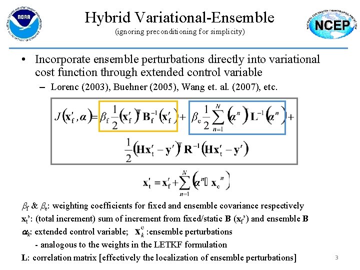
Hybrid Variational-Ensemble (ignoring preconditioning for simplicity) • Incorporate ensemble perturbations directly into variational cost function through extended control variable – Lorenc (2003), Buehner (2005), Wang et. al. (2007), etc. bf & be: weighting coefficients for fixed and ensemble covariance respectively xt’: (total increment) sum of increment from fixed/static B (xf’) and ensemble B ak: extended control variable; : ensemble perturbations - analogous to the weights in the LETKF formulation L: correlation matrix [effectively the localization of ensemble perturbations] 3

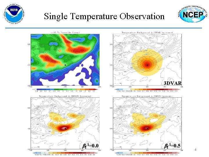
Single Temperature Observation 3 DVAR bf-1=0. 0 bf-1=0. 5 4

Outline • Introduction – (Brief) background on hybrid data assimilation • Hybrid Var/Ens at NCEP • OSSE-based hybrid experiments • Future Work and Summary 5

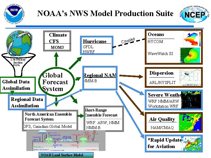
NOAA’s NWS Model Production Suite Climate CFS MOM 3 Hurricane GFDL HWRF led Coup Oceans HYCOM Wave. Watch III 1. 7 B Obs/Day Satellites 99. 9% Global Data Assimilation Global Forecast System Regional NAM NMM-B Regional Data Assimilation North American Ensemble Forecast System GFS, Canadian Global Model Dispersion ARL/HYSPLIT Severe Weather Short-Range Ensemble Forecast WRF: ARW, NMM-B WRF NMM/ARW Workstation WRF Air Quality NAM/CMAQ *Rapid Update for Aviation NOAH Land Surface Model For eca st 6

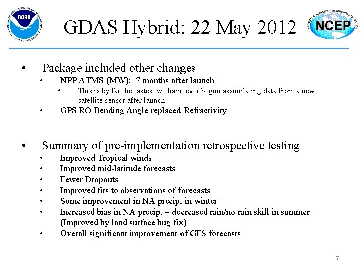
GDAS Hybrid: 22 May 2012 • Package included other changes • NPP ATMS (MW): 7 months after launch • • • This is by far the fastest we have ever begun assimilating data from a new satellite sensor after launch GPS RO Bending Angle replaced Refractivity Summary of pre-implementation retrospective testing • • Improved Tropical winds Improved mid-latitude forecasts Fewer Dropouts Improved fits to observations of forecasts Some improvement in NA precip. in winter Increased bias in NA precip. – decreased rain/no rain skill in summer (Improved by land surface bug fix) Overall significant improvement of GFS forecasts 7

TC Track Error Reduction HYBRID TEST GFS OPERATIONAL NHC/JTWC OFFICIAL 8

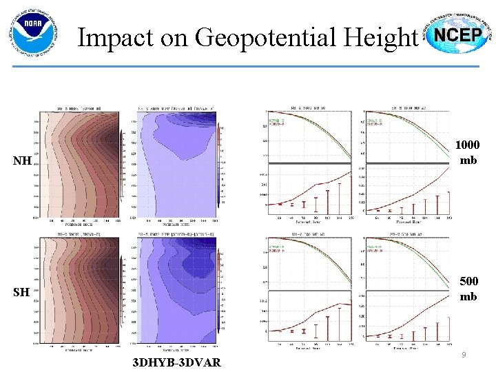
Impact on Geopotential Height NH 1000 mb SH 500 mb 3 DHYB-3 DVAR 9

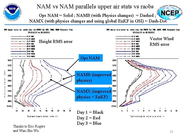
NAM vs NAM parallels upper air stats vs raobs Ops NAM = Solid ; NAMB (with Physics changes) = Dashed ; NAMX (with physics changes and using global En. KF in GSI) = Dash-Dot Vector Wind RMS error Height RMS error Ops NAMB (improved physics) NAMX (improved physics + En. KF) Thanks to Eric Rogers and Wan-Shu Wu Day 1 = Black Day 2 = Red Day 3 = Blue 10

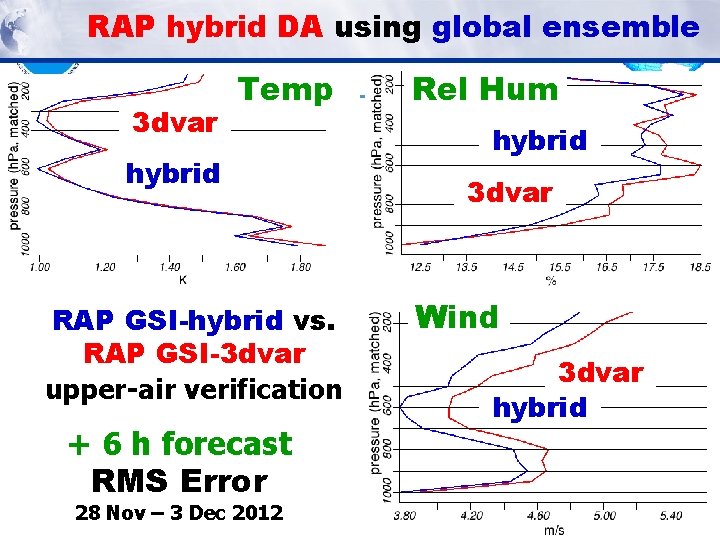
RAP hybrid DA using global ensemble 3 dvar Temp hybrid RAP GSI-hybrid vs. RAP GSI-3 dvar upper-air verification + 6 h forecast RMS Error 28 Nov – 3 Dec 2012 Rel Hum hybrid 3 dvar Wind 3 dvar hybrid

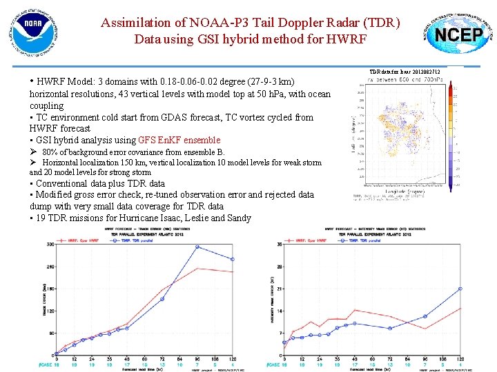
Assimilation of NOAA-P 3 Tail Doppler Radar (TDR) Data using GSI hybrid method for HWRF • HWRF Model: 3 domains with 0. 18 -0. 06 -0. 02 degree (27 -9 -3 km) horizontal resolutions, 43 vertical levels with model top at 50 h. Pa, with ocean coupling • TC environment cold start from GDAS forecast, TC vortex cycled from HWRF forecast • GSI hybrid analysis using GFS En. KF ensemble Ø 80% of background error covariance from ensemble B. Ø Horizontal localization 150 km, vertical localization 10 model levels for weak storm and 20 model levels for strong storm • Conventional data plus TDR data • Modified gross error check, re-tuned observation error and rejected data dump with very small data coverage for TDR data • 19 TDR missions for Hurricane Isaac, Leslie and Sandy TDR data for Isaac 2012082712

Outline • Introduction – (Brief) background on hybrid data assimilation • Hybrid Var/Ens at NCEP • OSSE-based hybrid experiments • Future Work and Summary 13

Observing System Simulation Experiments (OSSE) • Typically used to evaluate impact of future observing systems – Doppler-winds from spaced-based lidar, for example • Useful for evaluating present/proposed data assimilation techniques since ‘truth’ is known – Series of experiments are carried out to test hybrid variants • Joint OSSE – International, collaborative effort between ECMWF, NASA/GMAO, NOAA (NCEP/EMC, NESDIS, JCSDA), NOAA/ESRL, others – ECMWF-generated nature run (c 31 r 1) • T 511 L 91, 13 month free run, prescribed SST, snow, ice 14

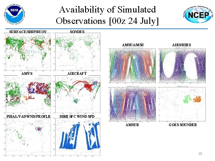
Availability of Simulated Observations [00 z 24 July] SURFACE/SHIP/BUOY SONDES AMSUA/MSU AMVS PIBAL/VADWND/PROFLR AIRS/HIRS AIRCRAFT SSMI SFC WIND SPD AMSUB GOES SOUNDER 15

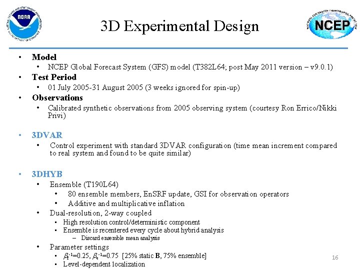
3 D Experimental Design • Model • • Test Period • • Calibrated synthetic observations from 2005 observing system (courtesy Ron Errico/Nikki Privi) 3 DVAR • • 01 July 2005 -31 August 2005 (3 weeks ignored for spin-up) Observations • • NCEP Global Forecast System (GFS) model (T 382 L 64; post May 2011 version – v 9. 0. 1) Control experiment with standard 3 DVAR configuration (time mean increment compared to real system and found to be quite similar) 3 DHYB • • Ensemble (T 190 L 64) • 80 ensemble members, En. SRF update, GSI for observation operators • Additive and multiplicative inflation Dual-resolution, 2 -way coupled • High resolution control/deterministic component • Ensemble is recentered every cycle about hybrid analysis – Discard ensemble mean analysis • Parameter settings • bf-1=0. 25, be-1=0. 75 [25% static B, 75% ensemble] • Level-dependent localization 16

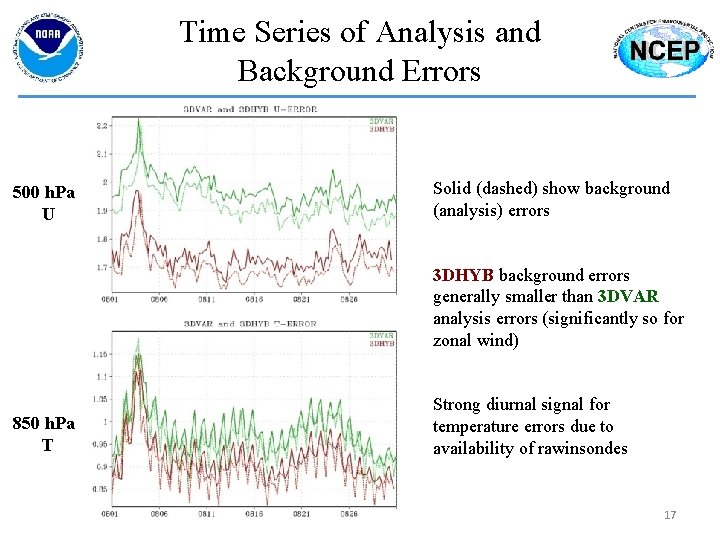
Time Series of Analysis and Background Errors 500 h. Pa U Solid (dashed) show background (analysis) errors 3 DHYB background errors generally smaller than 3 DVAR analysis errors (significantly so for zonal wind) 850 h. Pa T Strong diurnal signal for temperature errors due to availability of rawinsondes 17

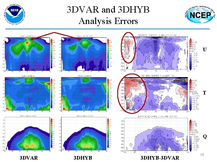
3 DVAR and 3 DHYB Analysis Errors U T Q 3 DVAR 3 DHYB-3 DVAR 18

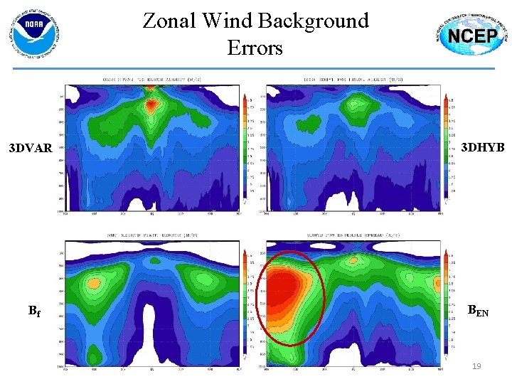
Zonal Wind Background Errors 3 DVAR Bf 3 DHYB BEN 19

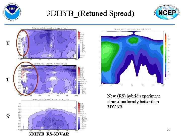
3 DHYB_(Retuned Spread) U T New (RS) hybrid experiment almost uniformly better than 3 DVAR Q 3 DHYB_RS-3 DVAR 20

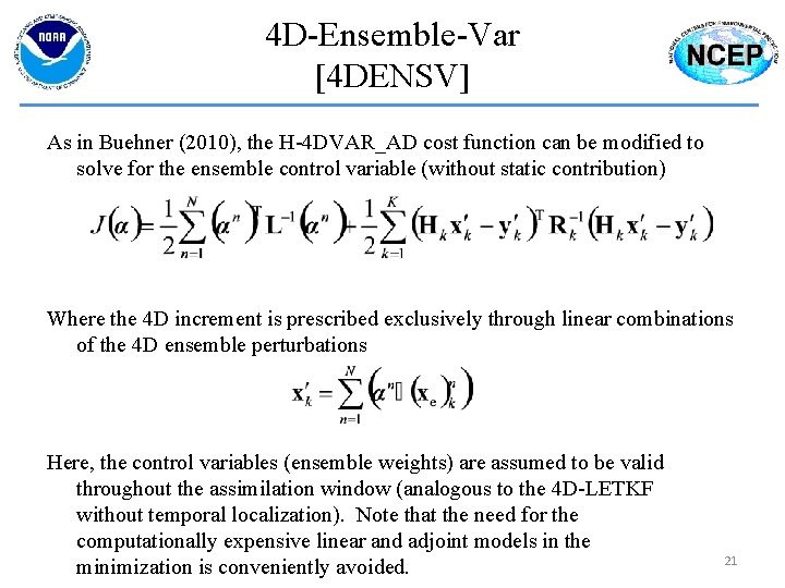
4 D-Ensemble-Var [4 DENSV] As in Buehner (2010), the H-4 DVAR_AD cost function can be modified to solve for the ensemble control variable (without static contribution) Where the 4 D increment is prescribed exclusively through linear combinations of the 4 D ensemble perturbations Here, the control variables (ensemble weights) are assumed to be valid throughout the assimilation window (analogous to the 4 D-LETKF without temporal localization). Note that the need for the computationally expensive linear and adjoint models in the minimization is conveniently avoided. 21

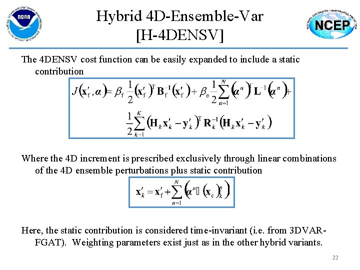
Hybrid 4 D-Ensemble-Var [H-4 DENSV] The 4 DENSV cost function can be easily expanded to include a static contribution Where the 4 D increment is prescribed exclusively through linear combinations of the 4 D ensemble perturbations plus static contribution Here, the static contribution is considered time-invariant (i. e. from 3 DVARFGAT). Weighting parameters exist just as in the other hybrid variants. 22

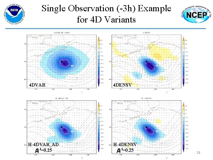
Single Observation (-3 h) Example for 4 D Variants 4 DVAR 4 DENSV H-4 DVAR_AD bf-1=0. 25 H-4 DENSV bf-1=0. 25 23

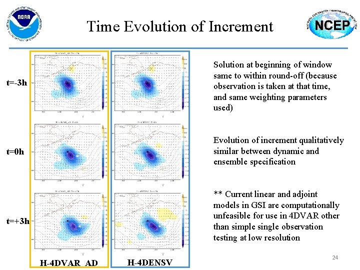
Time Evolution of Increment t=-3 h Solution at beginning of window same to within round-off (because observation is taken at that time, and same weighting parameters used) t=0 h Evolution of increment qualitatively similar between dynamic and ensemble specification ** Current linear and adjoint models in GSI are computationally unfeasible for use in 4 DVAR other than simple single observation testing at low resolution t=+3 h H-4 DVAR_AD H-4 DENSV 24

4 D OSSE Experiments • To investigate the use of 4 D ensemble perturbations, two new OSSE based experiments are carried out. • The original (not reduced) set of inflation parameters are used. • Exact configuration as was used in the 3 D OSSE experiments, but with 4 D features – 4 DENSV • No static B contribution (bf-1=0. 0) • Analogous to a dual-resolution 4 D-En. KF (but solved variationally) • To be compared with 3 DENSV – H-4 DENSV • 4 DENSV + addition of time invariant static contribution (bf-1=0. 25) • This is the non-adjoint formulation • To be compared with 4 DENSV 25

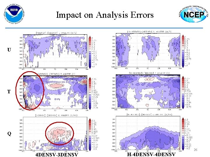
Impact on Analysis Errors U T Q 4 DENSV-3 DENSV H-4 DENSV 26

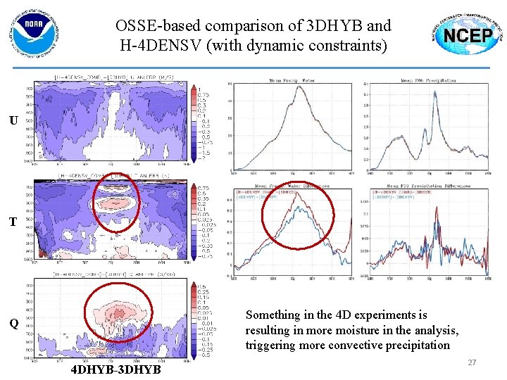
OSSE-based comparison of 3 DHYB and H-4 DENSV (with dynamic constraints) U T Something in the 4 D experiments is resulting in more moisture in the analysis, triggering more convective precipitation Q 4 DHYB-3 DHYB 27

Summary of 4 D Experiments • 4 DENSV seems to be a cost effective alternative to 4 DVAR • Inclusion of time-invariant static B to 4 DENSV solution is beneficial for dual-resolution paradigm • Extension to 4 D seems to have larger impact in extratropics (whereas the original introduction of the ensemble covariances had largest impact in the tropics) • Increased convection in 4 D extensions remains a mystery (it is not the weak constraint on unphysical moisture as I originally hypothesized) • Original tuning parameters for inflation were utilized. Follow-on experiments with tuned parameters (reduced inflation) and/or adapative inflation should yield even more impressive results. 28

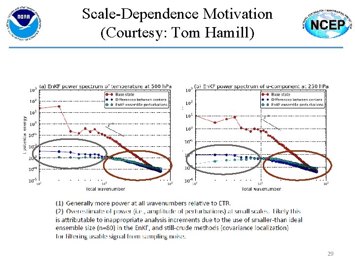
Scale-Dependence Motivation (Courtesy: Tom Hamill) 29

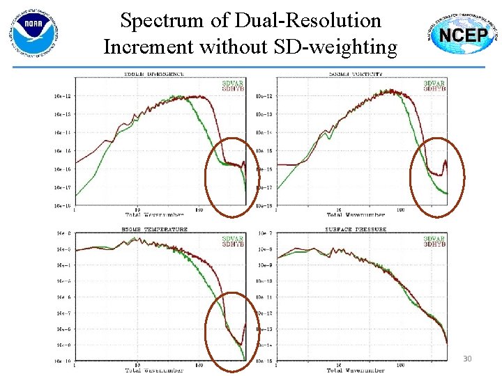
Spectrum of Dual-Resolution Increment without SD-weighting 30

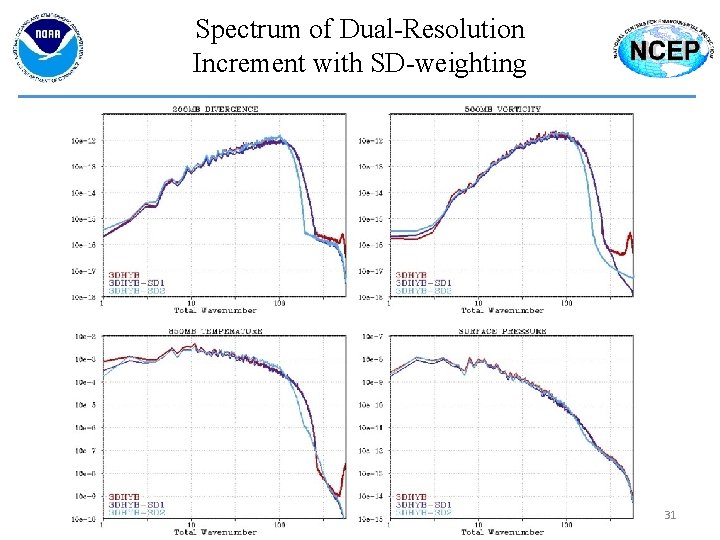
Spectrum of Dual-Resolution Increment with SD-weighting 31

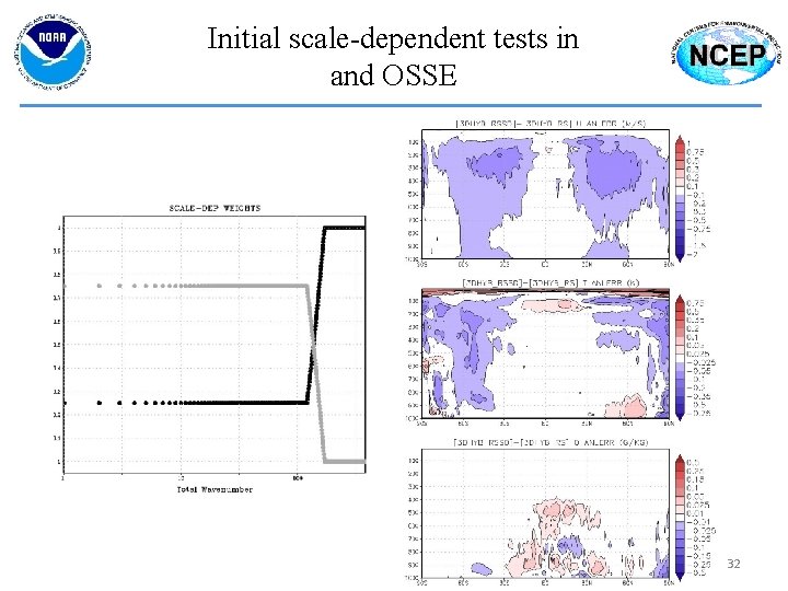
Initial scale-dependent tests in and OSSE 32

Outline • Introduction – (Brief) background on hybrid data assimilation • Hybrid Var/Ens at NCEP • OSSE-based hybrid experiments • Future Work and Summary 33

Summary • NCEP successfully implemented hybrid variational-ensemble algorithm into GDAS • NCEP aggressively pursuing application of hybrid to other systems – Mesoscale (NAM), HWRF, Rapid Refresh (and HRRR follow on), storm scale ensemble – Future Reanalysis • Have already run preliminary tests for 1981 -1983 periods, attempting to capture QBO transitions (a difficult problem for reduced observing system periods) • Extensions to the GDAS hybrid are ongoing, including 4 DEns. Var 34

GDAS Hybrid • EMC targeting T 1148 SL GFS implementation within next year – How to configure hybrid? What can be afforded computationally on new machine? • Merging DA and EPS efforts – Currently have separate En. KF (DA) and BV-ETR (EPS) cycles/perturbations • Improving the ensemble for the hybrid – Stochastic physics (Jeff Whitaker) – TC Initialization (Yoichiro Ota) • Hybrid developments – Improved localization, flow-dependent (and/or scale-dependent) weighting – Testing and preparing 4 d-ensemble-var for implementation – Helping efforts toward cloudy/precip. radiances 35

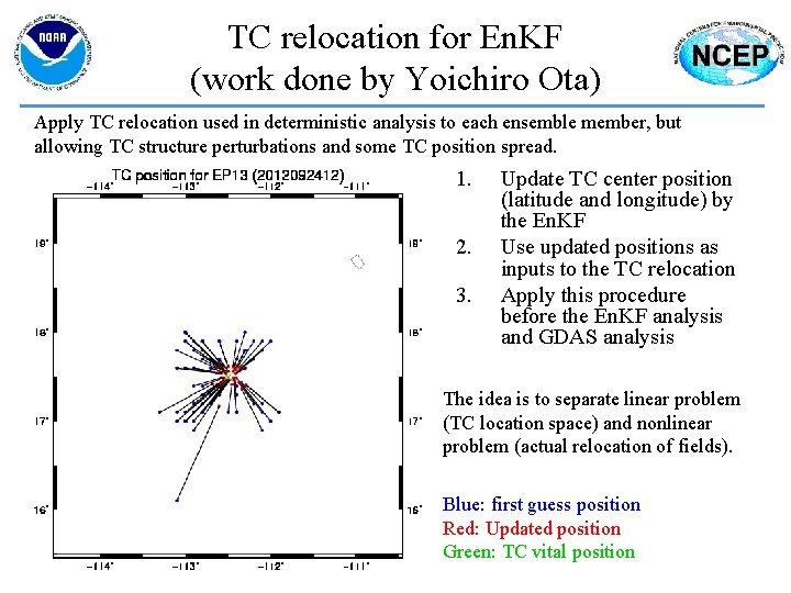
TC relocation for En. KF (work done by Yoichiro Ota) Apply TC relocation used in deterministic analysis to each ensemble member, but allowing TC structure perturbations and some TC position spread. 1. 2. 3. Update TC center position (latitude and longitude) by the En. KF Use updated positions as inputs to the TC relocation Apply this procedure before the En. KF analysis and GDAS analysis The idea is to separate linear problem (TC location space) and nonlinear problem (actual relocation of fields). Blue: first guess position Red: Updated position Green: TC vital position

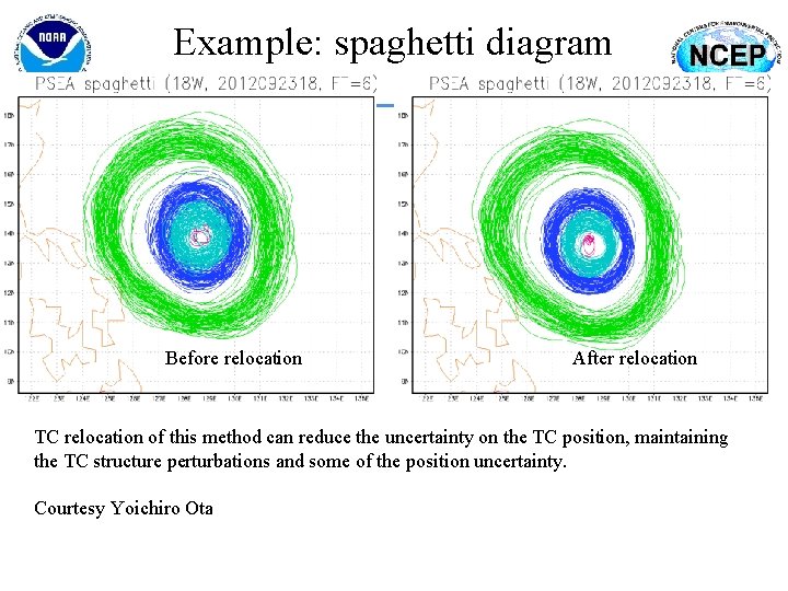
Example: spaghetti diagram Before relocation After relocation TC relocation of this method can reduce the uncertainty on the TC position, maintaining the TC structure perturbations and some of the position uncertainty. Courtesy Yoichiro Ota

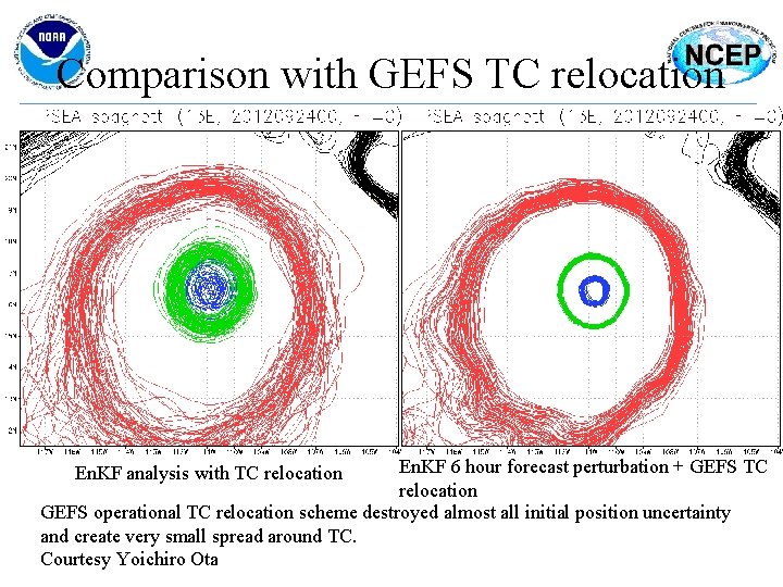
Comparison with GEFS TC relocation En. KF 6 hour forecast perturbation + GEFS TC relocation GEFS operational TC relocation scheme destroyed almost all initial position uncertainty and create very small spread around TC. Courtesy Yoichiro Ota En. KF analysis with TC relocation

6 th WMO Symposium on DA • NCEP will be hosting the next WMO DA Symposium from 7 -11 October 2013 at NCWCP • Call for papers will be out soon 39

• BACKUP SLIDES 40

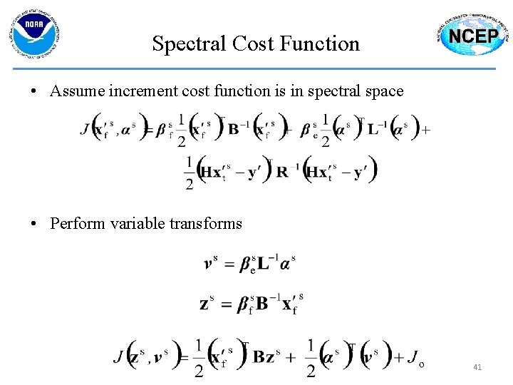
Spectral Cost Function • Assume increment cost function is in spectral space • Perform variable transforms 41

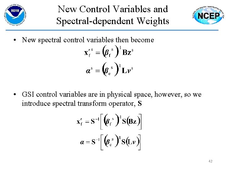
New Control Variables and Spectral-dependent Weights • New spectral control variables then become • GSI control variables are in physical space, however, so we introduce spectral transform operator, S 42

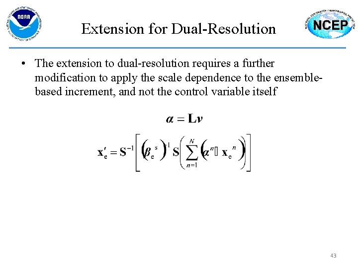
Extension for Dual-Resolution • The extension to dual-resolution requires a further modification to apply the scale dependence to the ensemblebased increment, and not the control variable itself 43