Human Animal and Machine Learning Vasile Rus http

Human, Animal, and Machine Learning Vasile Rus http: //www. cs. memphis. edu/~vrus/teaching/cogsci

Overview • Evaluating Hypotheses

Overview of the lecture • Evaluating Hypotheses (errors, accuracy) • Comparing Hypotheses • Comparing Learning Algorithms (hold-out methods) • Performance Measures

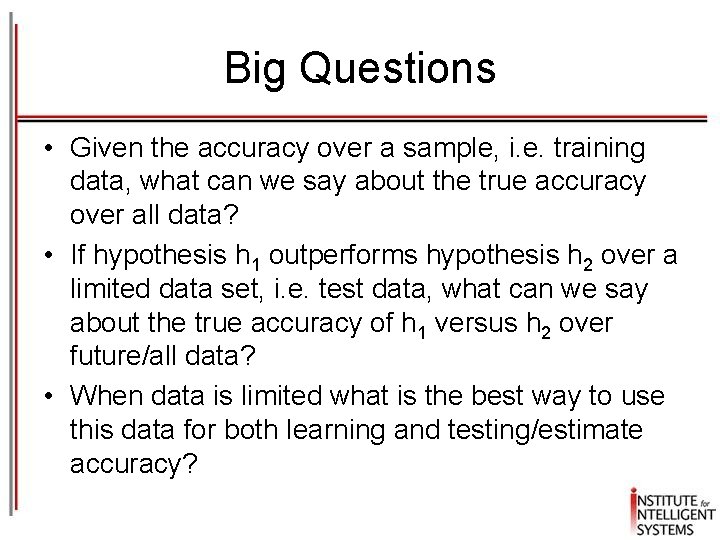
Big Questions • Given the accuracy over a sample, i. e. training data, what can we say about the true accuracy over all data? • If hypothesis h 1 outperforms hypothesis h 2 over a limited data set, i. e. test data, what can we say about the true accuracy of h 1 versus h 2 over future/all data? • When data is limited what is the best way to use this data for both learning and testing/estimate accuracy?

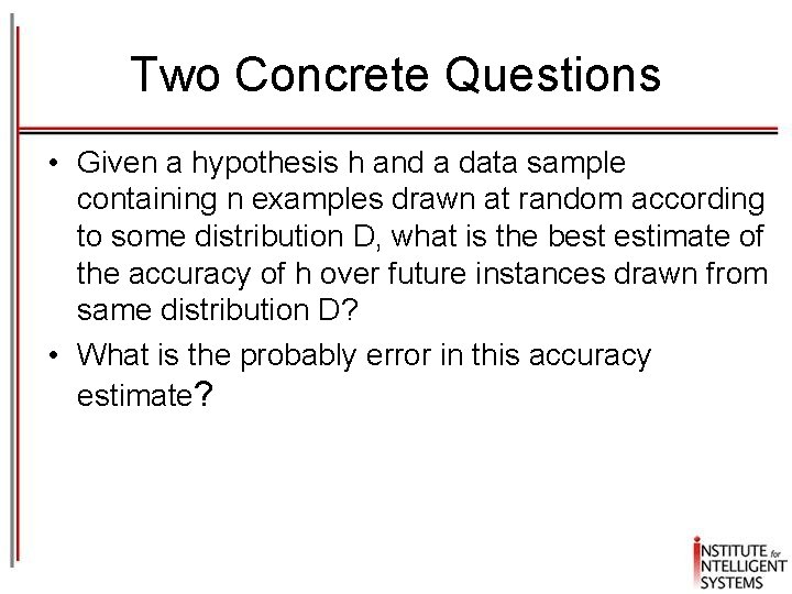
Two Concrete Questions • Given a hypothesis h and a data sample containing n examples drawn at random according to some distribution D, what is the best estimate of the accuracy of h over future instances drawn from same distribution D? • What is the probably error in this accuracy estimate?

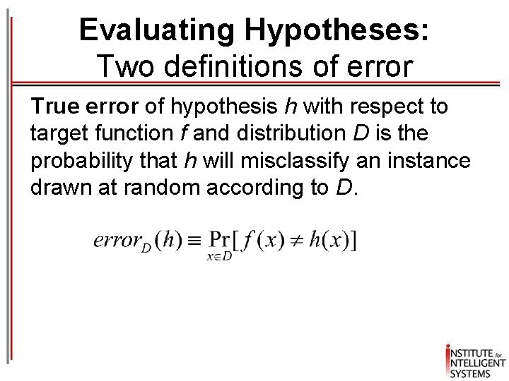
Evaluating Hypotheses: Two definitions of error True error of hypothesis h with respect to target function f and distribution D is the probability that h will misclassify an instance drawn at random according to D.

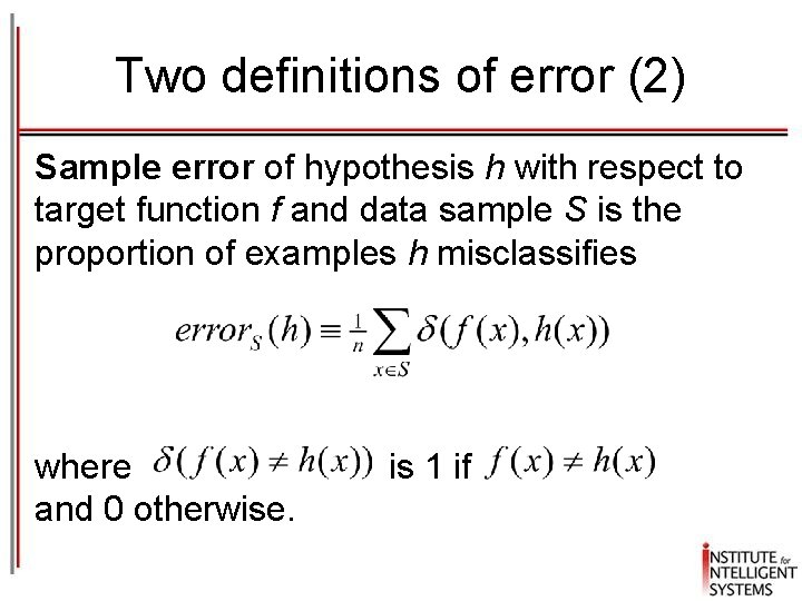
Two definitions of error (2) Sample error of hypothesis h with respect to target function f and data sample S is the proportion of examples h misclassifies where is 1 if and 0 otherwise.

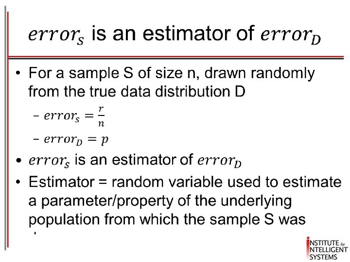
How good an estimate of true error. D(h) (which we wish to know) is sample error. S(h) (which we can observer/measure)?

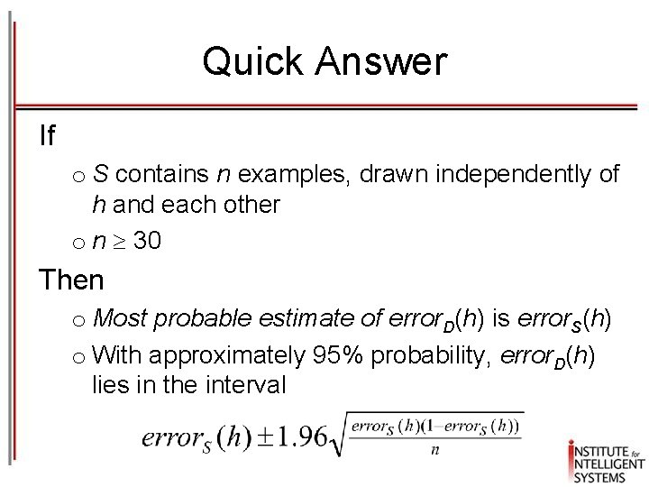
Quick Answer If o S contains n examples, drawn independently of h and each other o n 30 Then o Most probable estimate of error. D(h) is error. S(h) o With approximately 95% probability, error. D(h) lies in the interval

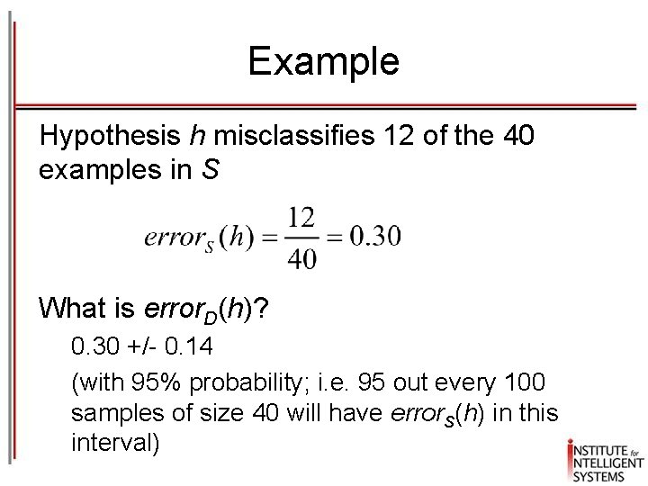
Example Hypothesis h misclassifies 12 of the 40 examples in S What is error. D(h)? 0. 30 +/- 0. 14 (with 95% probability; i. e. 95 out every 100 samples of size 40 will have error. S(h) in this interval)

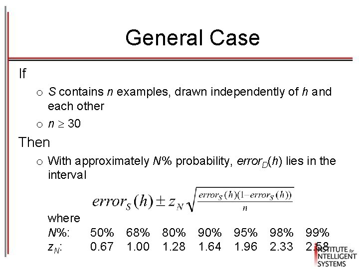
General Case If o S contains n examples, drawn independently of h and each other o n 30 Then o With approximately N% probability, error. D(h) lies in the interval where N%: 50% 68% 80% 95% 98% 99% z. N: 0. 67 1. 00 1. 28 1. 64 1. 96 2. 33 2. 58

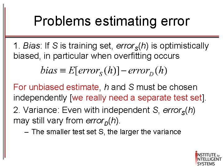
Problems estimating error 1. Bias: If S is training set, error. S(h) is optimistically biased, in particular when overfitting occurs For unbiased estimate, h and S must be chosen independently [we really need a separate test set]. 2. Variance: Even with independent S, error. S(h) may still vary from error. D(h). – The smaller test set S, the larger the variance

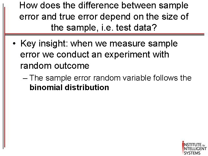
How does the difference between sample error and true error depend on the size of the sample, i. e. test data? • Key insight: when we measure sample error we conduct an experiment with random outcome – The sample error random variable follows the binomial distribution

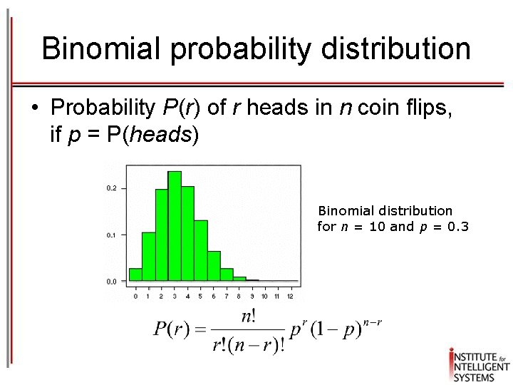
Binomial probability distribution • Probability P(r) of r heads in n coin flips, if p = P(heads) Binomial distribution for n = 10 and p = 0. 3

Binomial probability distribution • Expected, or mean value of X, E[X], is • Variance of X is • Standard deviation of X, is

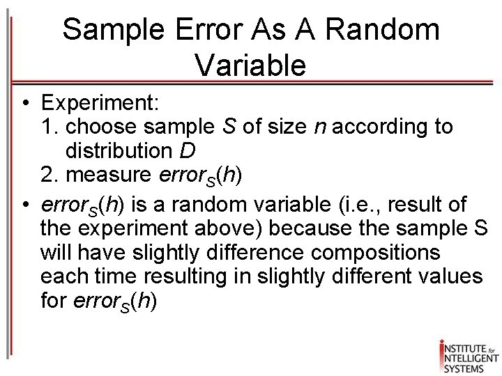
Sample Error As A Random Variable • Experiment: 1. choose sample S of size n according to distribution D 2. measure error. S(h) • error. S(h) is a random variable (i. e. , result of the experiment above) because the sample S will have slightly difference compositions each time resulting in slightly different values for error. S(h)

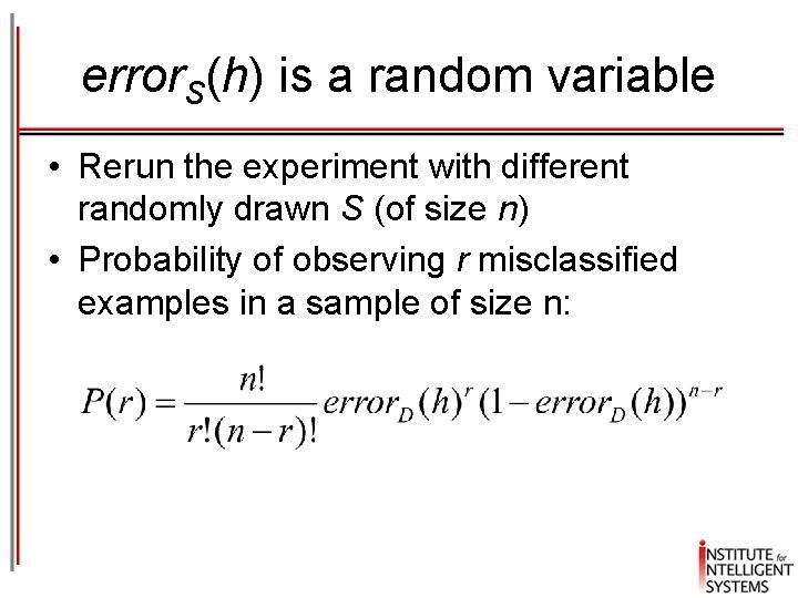
error. S(h) is a random variable • Rerun the experiment with different randomly drawn S (of size n) • Probability of observing r misclassified examples in a sample of size n:

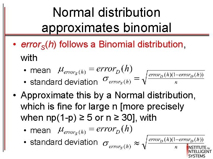
Normal distribution approximates binomial • error. S(h) follows a Binomial distribution, with • mean • standard deviation • Approximate this by a Normal distribution, which is fine for large n [more precisely when np(1 -p) ≥ 5 or n ≥ 30], with • mean • standard deviation

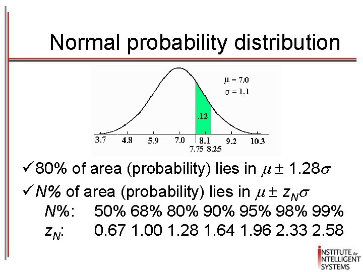
Normal probability distribution ü 80% of area (probability) lies in 1. 28 ü N% of area (probability) lies in z. N N%: 50% 68% 80% 95% 98% 99% z. N: 0. 67 1. 00 1. 28 1. 64 1. 96 2. 33 2. 58

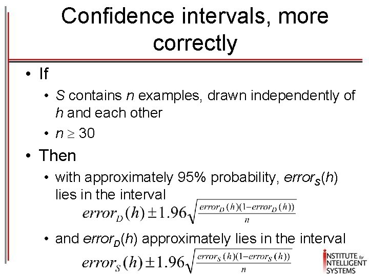
Confidence intervals, more correctly • If • S contains n examples, drawn independently of h and each other • n 30 • Then • with approximately 95% probability, error. S(h) lies in the interval • and error. D(h) approximately lies in the interval

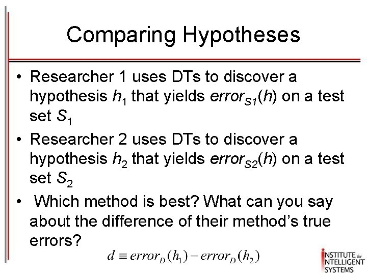
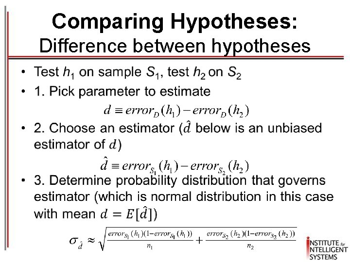
Comparing Hypotheses • Researcher 1 uses DTs to discover a hypothesis h 1 that yields error. S 1(h) on a test set S 1 • Researcher 2 uses DTs to discover a hypothesis h 2 that yields error. S 2(h) on a test set S 2 • Which method is best? What can you say about the difference of their method’s true errors?

Comparing Hypotheses: Difference between hypotheses •

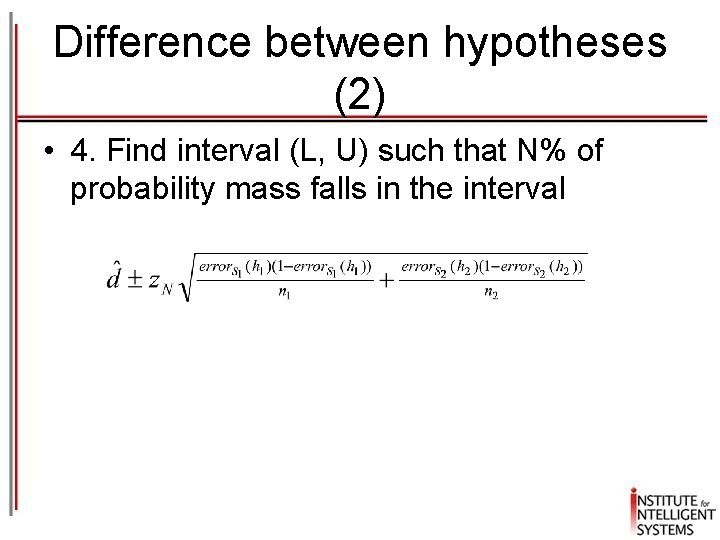
Difference between hypotheses (2) • 4. Find interval (L, U) such that N% of probability mass falls in the interval

Comparing Learning Algorithms • Researcher 1 uses DTs to learn some target function f • Researcher 2 uses Perceptron to learn same target function f • Which learning algorithm is best on average?

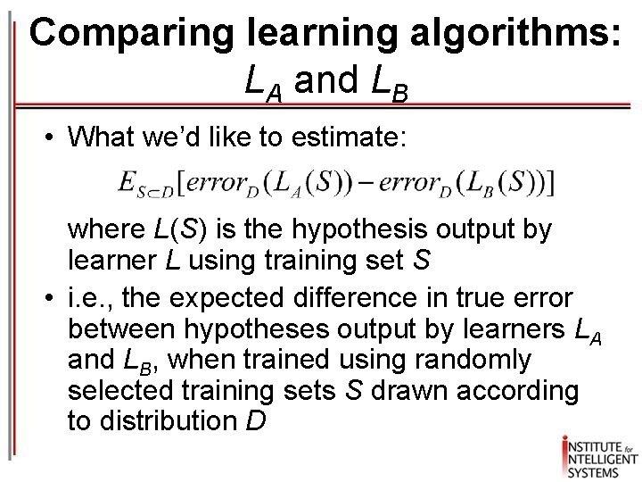
Comparing learning algorithms: LA and LB • What we’d like to estimate: where L(S) is the hypothesis output by learner L using training set S • i. e. , the expected difference in true error between hypotheses output by learners LA and LB, when trained using randomly selected training sets S drawn according to distribution D

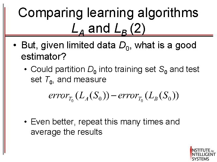
Comparing learning algorithms LA and LB (2) • But, given limited data D 0, what is a good estimator? • Could partition D 0 into training set S 0 and test set T 0, and measure • Even better, repeat this many times and average the results

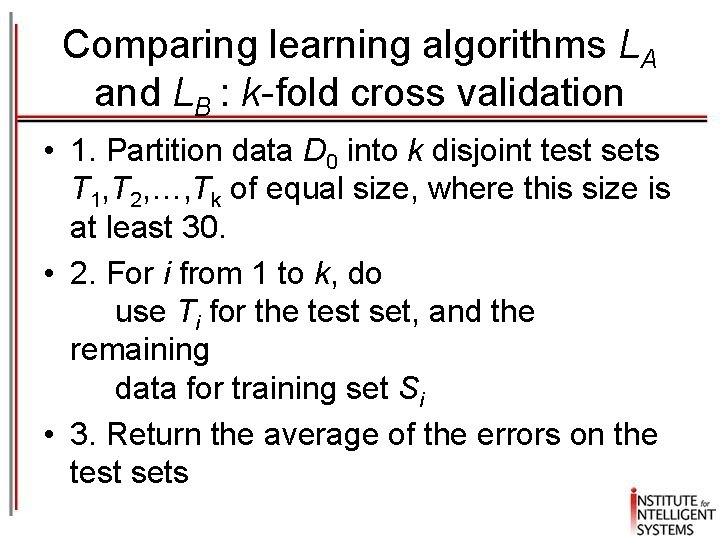
Comparing learning algorithms LA and LB : k-fold cross validation • 1. Partition data D 0 into k disjoint test sets T 1, T 2, …, Tk of equal size, where this size is at least 30. • 2. For i from 1 to k, do use Ti for the test set, and the remaining data for training set Si • 3. Return the average of the errors on the test sets

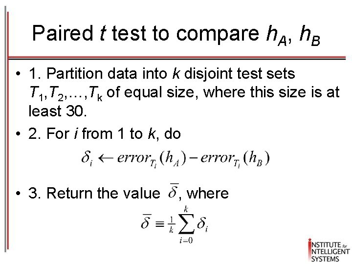
Paired t test to compare h. A, h. B • 1. Partition data into k disjoint test sets T 1, T 2, …, Tk of equal size, where this size is at least 30. • 2. For i from 1 to k, do • 3. Return the value , where

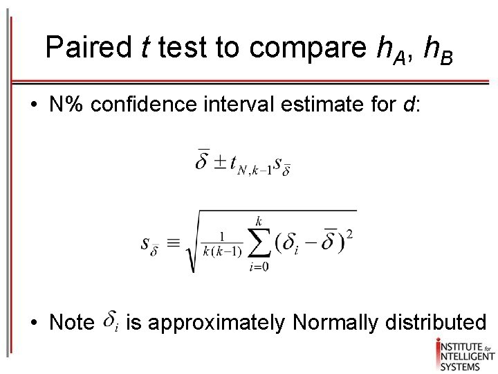
Paired t test to compare h. A, h. B • N% confidence interval estimate for d: • Note is approximately Normally distributed

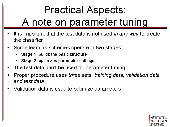
Practical Aspects: A note on parameter tuning • It is important that the test data is not used in any way to create the classifier • Some learning schemes operate in two stages: • Stage 1: builds the basic structure • Stage 2: optimizes parameter settings • The test data can’t be used for parameter tuning! • Proper procedure uses three sets: training data, validation data, and test data • Validation data is used to optimize parameters

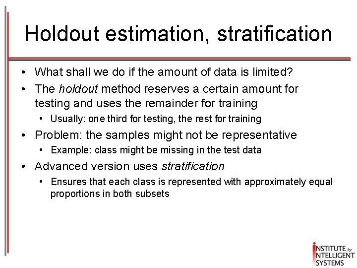
Holdout estimation, stratification • What shall we do if the amount of data is limited? • The holdout method reserves a certain amount for testing and uses the remainder for training • Usually: one third for testing, the rest for training • Problem: the samples might not be representative • Example: class might be missing in the test data • Advanced version uses stratification • Ensures that each class is represented with approximately equal proportions in both subsets

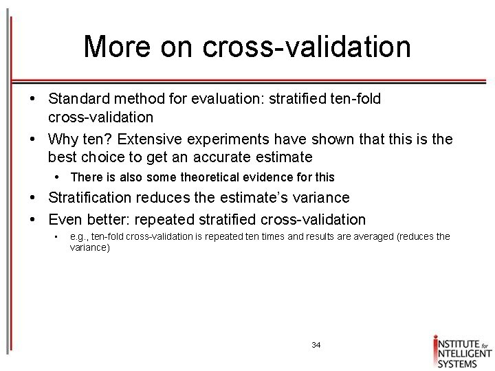
More on cross-validation • Standard method for evaluation: stratified ten-fold cross-validation • Why ten? Extensive experiments have shown that this is the best choice to get an accurate estimate • There is also some theoretical evidence for this • Stratification reduces the estimate’s variance • Even better: repeated stratified cross-validation • e. g. , ten-fold cross-validation is repeated ten times and results are averaged (reduces the variance) 34

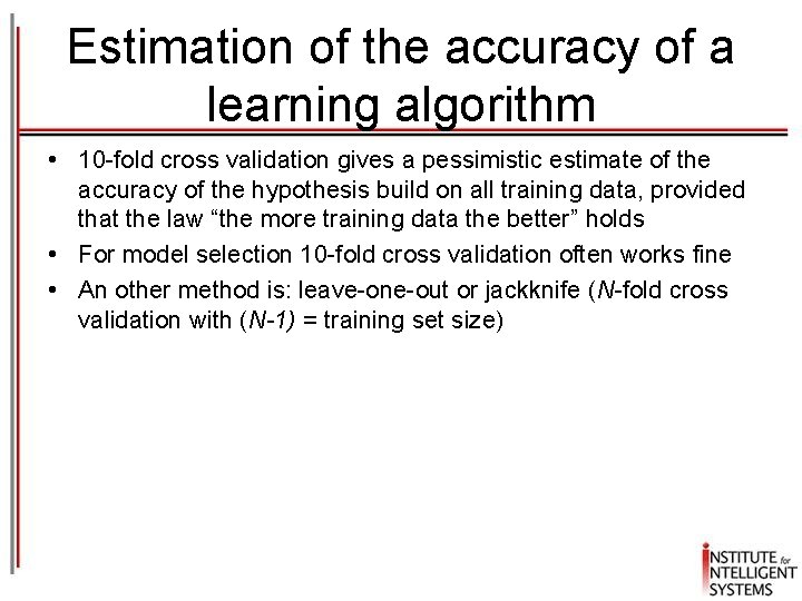
Estimation of the accuracy of a learning algorithm • 10 -fold cross validation gives a pessimistic estimate of the accuracy of the hypothesis build on all training data, provided that the law “the more training data the better” holds • For model selection 10 -fold cross validation often works fine • An other method is: leave-one-out or jackknife (N-fold cross validation with (N-1) = training set size)

Model selection criteria • Model selection criteria attempt to find a good compromise between: A. The complexity of a model B. Its prediction accuracy on the training data • Reasoning: a good model is a simple model that achieves high accuracy on the given data • Also known as Occam’s Razor: the best theory is the smallest one that describes all the facts

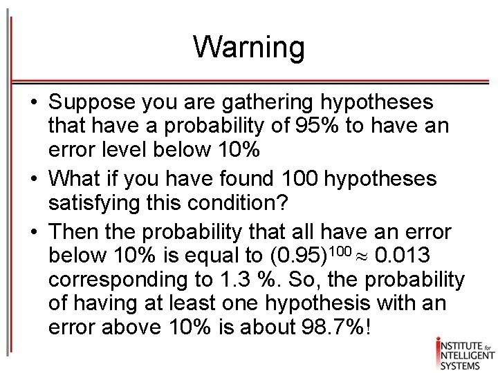
Warning • Suppose you are gathering hypotheses that have a probability of 95% to have an error level below 10% • What if you have found 100 hypotheses satisfying this condition? • Then the probability that all have an error below 10% is equal to (0. 95)100 0. 013 corresponding to 1. 3 %. So, the probability of having at least one hypothesis with an error above 10% is about 98. 7%!

No Free Lunch Theorem!!! • Theorem (no free lunch) • For any two learning algorithms LA and LB the following is true, independently of the sampling distribution and the number of training instances n: • Uniformly averaged over all target functions F, E(error. S(h. A) | F, n) = E(error. S(h. B) | F, n) • Same for a fixed training set D

No Free Lunch • The other way around: for any ML algorithm there exist data sets on which it performs well and there exist data sets on which it performs badly! • We hope that the latter sets do not occur too often in real life

Summary • Evaluating Hypotheses

Next Time • Bayesian Learning