HST 582 6 555 Image Processing II 2

HST 582 / 6. 555 Image Processing II

2 D and 3 D Image Processing • Useful linear signal processing for medical images – Interpolation – Down sampling – Hierarchical filtering – Computed Tomography (CT), • Projection Slice Theorem

2 D and 3 D Image Processing • Useful non-linear processing techniques – Histogram equalization – Homomorphic filtering – Gradient limited diffusion – Edge detection

Applications of Signal Processing in Medical Images • Linear signal processing – Image reconstruction (tomography, MRI) – Image enhancement – Noise reduction – Artifact reduction • Non-linear signal processing – Non-linear, adaptive filters • Tube enhancing filters

Interpolating Images • Why – Prepare synthetic multichannel data – Prepare data sets for parallel trips down the same processing pipeline

Interpolation • Optimal – Reconstruct the bandlimited original signal using sinc functions – Re-sample the reconstruction • Nearest Neighbor • Linear

Nearest Neighbor • Easy interpolator I 11 I 21 I 31 I 22 I 32 I 12 … … – To interpolate here, assign the intensity of the closest original pixel (in this case, I 11) – leads to blocky results

Linear Interpolator (1 D) f 2 f 1 0 f( T) = f 1 + T (f 2 - f 1) T 1

Bilinear Interpolator (2 D) • 2 D linear interpolator f 11 A f 21 C f 12 B use 1 D linear interpolation for A and B, use 1 D linear interpolation among A and B to get C • Similar for 3 D f 22

Bilinear Interpolator. . . T 1 f 11 A f 21 C f 12 B f 22 T 2 f( T 1, T 2) = f 11 + T 1 (f 21 - f 11) + T 2 (f 12 - f 11) + T 1 T 2 (f 22 - f 21 - f 12 + f 11)

Down Sampling • If you are lowpass filtering, maybe you can discard alternating pixels with losing too much • If you want to down-sample, maybe you should first do some lowpass filter to avoid aliasing – Reasonable LPF to use:

Burt (Peter) Filter image lowpass filter decimate by 2 ½ size image ¼ size image 1/ 8 size image

Projection Slice Theorem and CT x-rays Focus on one ray: (discrete) source … sensor photons leaving = An • photons entering

Continuous Analog. . . x is a log-attenuation-density called: Linear Attenuation Coefficient x(t 1, t 2) t 1 t 2 we can model x-ray imaging by line integrals…

Fourier Transform. . . x(t 1, t 2) Transform pairs xp(t 1) Transform pairs

CT Reconstruction using FT Methods • Rotate the x-ray apparatus to many angles – Take projections • FT the projections • Assemble the transformed projections in frequency space: – Get frequency data on these lines at the angles the projections were taken • Interpolate the full frequency space • Inverse FT to get back reconstruction There is a related method: Filtered Back-projection which is usually used

Linear and Non-Linear Processing for Medical Images Data Reconstruct image: usually linear image Improve image: maybe linear better image Segment, find surfaces: non-linear

Histogram Equalization • A method for automatically setting intensity lookup table • Apply a monotonic transformation to the data so that after the transformation, the result has a (nearly) uniform intensity histogram • Tends to increase contrast in areas where the data is concentrated

Histogram the Image Intensities Data Desired Histogram 0 Cumulative Data 255 Desired Cumulative 0 L A H 0 B 255

Histogram: Examples Image and its intensity histogram Histogram equalization From Lim

Homomorphic Filtering • An automatic method for spatially varying contrast adjustment <1 lowpass exp log highpass >1 H( ) ( 12+ 22)

Homomorphic Processing: Example Original image related: unsharp masking Image after homomorphic processing From Lim

Boundary Preserving Smoothers • “Gradient Limited Diffusion” –Malik & Perona – Currently the method of choice for postprocessing MRI before 3 D graphics.

Diffusion time • In GLD the diffusivity is moderated by the gradient magnitude, and the simulation is run for finite time.

Duality • Focus on regions Segmentation • Focus on boundaries Edges • Sometimes best to do both.

Edge Detection • From computer vision – Roberts – Horn – Marr and Hildreth – Canny Picture 1965 1972 1980 1983 Lincoln Lab MIT AI Higher Processor a compact description

Basic Idea: 1 D Edge • Motivation: ideal step edge + noise intensity this is the important information space 1 st find peak derivative space

Edges in 2 D profile • Strategy: – Find direction of gradient contour lines – Analyze derivative of signal in direction of gradients

Zero Crossing Style Edges: 1 D signal peak 1 st derivative 2 nd derivative Mark edges where 2 nd derivative = 0 (vigorously) zero crossing

Noise • Noise is an issue with derivative operators – How do we fight the noise • Assume white noise • Assume good stuff has important low frequency content • recall Wiener filtering. . .

Noise • Noise is an issue with derivative operators – How do we fight the noise • Assume white noise • Assume good stuff has important low frequency content • USE LOWPASS FILTER (Gaussian ? )

Difference of Gaussians Gaussian Blur signal 2 nd Derivative + mark zero crossings

Works in 2 D, 3 D, … • Gaussian separates • There exists a rotationally-symmetric 2 nd derivative operator: Laplacian similar for 3 D Discrete analog: -1 -1 -1 8 -1 -1 -1

2 D 2 G Operator • The zero crossing contours of the result of an operator like this form closed contours. “Mexican hat”

Seminal Edge References. . . • “Theory of Edge Detection”, David Marr, Ellen Hildreth, Proc. Royal Statistical Society of London, B, vol 207, pp 187 -217, 1980 – good paper, often cited • VISION, David Marr – good book!

Threshold Bug • Excess zero crossings from noise, etc. – Usual fix: threshold edges based on “strength. ”

Edge Detection In 2 D: threshold based on gradient strength signal big 1 st derivative magnitude 1 st derivative 2 nd derivative “strong” zero crossing

(Pen)ultimate Edge Operator Canny • For improved noise behavior go back to 1 D directional derivatives • For less fragmentation – Use Hysteresis thresholding • The problem: edge fragmentation

In 1 D Along 2 D Contour threshold edge strength

Schmidt Trigger uses Hysteresis High threshold Low Threshold edge strength

John Canny MIT MS Thesis

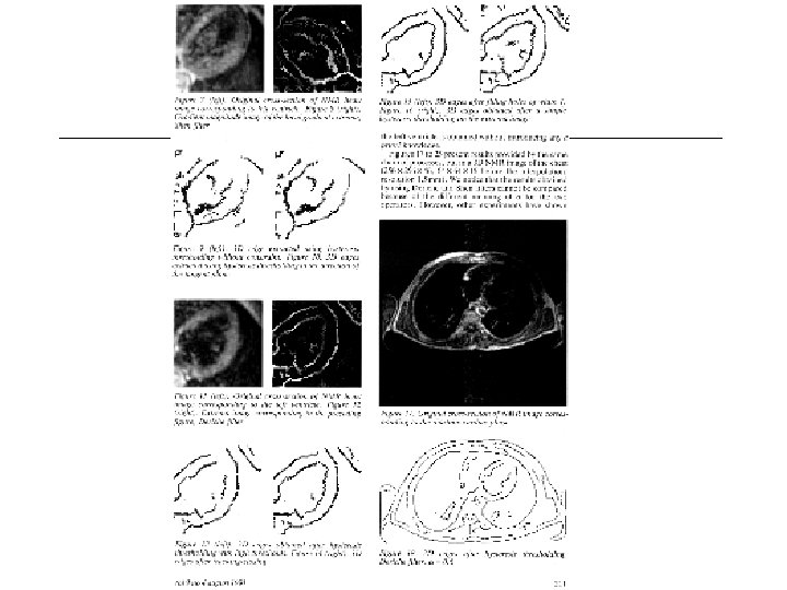
Edge Detection: Example Original image

Edge Detection: Example Detected edges

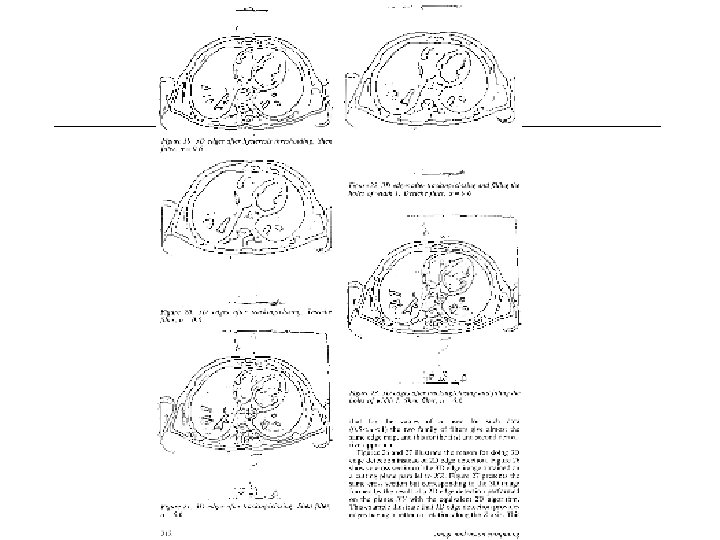
Edges in 3 D are Surfaces • Somewhat useful for finding organ boundaries (e. g. in CT). – Simple. – May leave the problem of figuring out which boundary is what.

3 D Medical Edge Finding. . . • Recursive Filtering and Edge Tracking: Two Primary Tools for 3 D Edge Detection – Olivier Monga, Rachid Deriche, Gergoire Malandain, Jean Pierre Cocquerez – Image and Vision Computing Vol 9, Nr. 4, 1991

the end.