How to plot the Fermi surface using SIESTA

How to plot the Fermi surface using SIESTA and WANNIER 90 Javier Junquera

We are going to plot the Fermi surface of electron-doped bulk Sr. Ti. O 3 To charge slightly the bulk unit cell of Sr. Ti. O 3, introduce the following line in the input file Net. Charge -0. 10 Then, follow step by step all the process described in the exercise about the Wannier functions

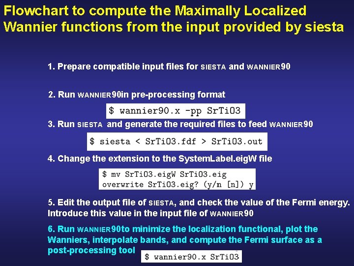
Flowchart to compute the Maximally Localized Wannier functions from the input provided by siesta 1. Prepare compatible input files for SIESTA and WANNIER 90 2. Run WANNIER 90 in pre-processing format 3. Run SIESTA and generate the required files to feed WANNIER 90 4. Change the extension to the System. Label. eig. W file 5. Run WANNIER 90 to minimize the localization functional, plot the Wanniers, interpolate bands, etc as a post-processing tool

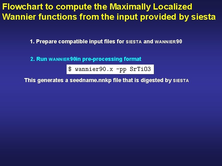
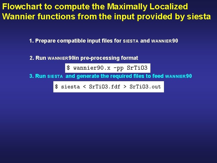
Flowchart to compute the Maximally Localized Wannier functions from the input provided by siesta 1. Prepare compatible input files for SIESTA and WANNIER 90 2. Run WANNIER 90 in pre-processing format This generates a seedname. nnkp file that is digested by SIESTA

Flowchart to compute the Maximally Localized Wannier functions from the input provided by siesta 1. Prepare compatible input files for SIESTA and WANNIER 90 2. Run WANNIER 90 in pre-processing format 3. Run SIESTA and generate the required files to feed WANNIER 90

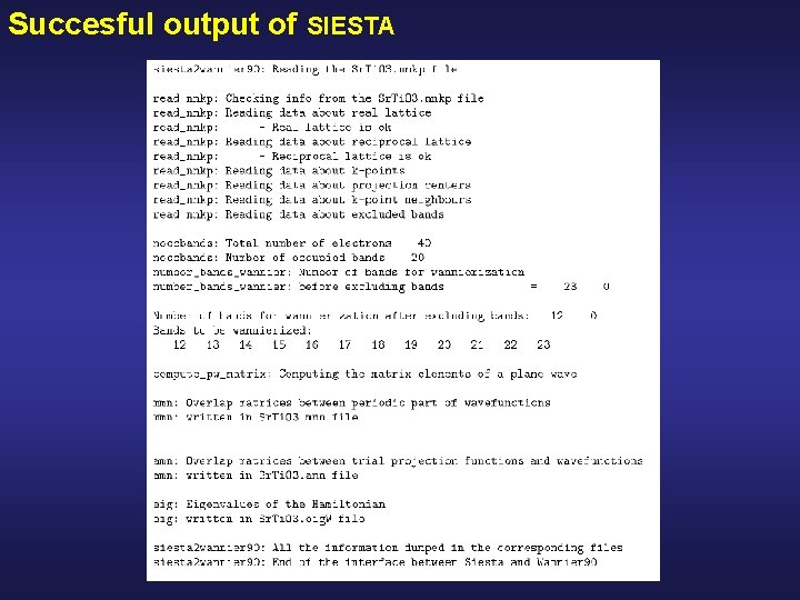
Succesful output of SIESTA

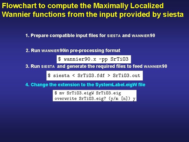
Flowchart to compute the Maximally Localized Wannier functions from the input provided by siesta 1. Prepare compatible input files for SIESTA and WANNIER 90 2. Run WANNIER 90 in pre-processing format 3. Run SIESTA and generate the required files to feed WANNIER 90 4. Change the extension to the System. Label. eig. W file

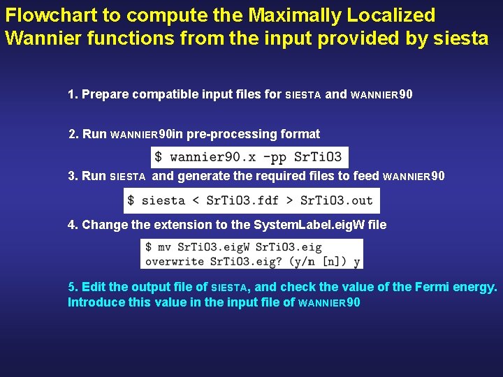
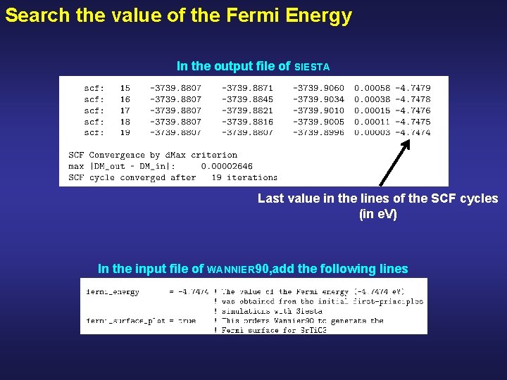
Flowchart to compute the Maximally Localized Wannier functions from the input provided by siesta 1. Prepare compatible input files for SIESTA and WANNIER 90 2. Run WANNIER 90 in pre-processing format 3. Run SIESTA and generate the required files to feed WANNIER 90 4. Change the extension to the System. Label. eig. W file 5. Edit the output file of SIESTA, and check the value of the Fermi energy. Introduce this value in the input file of WANNIER 90

Search the value of the Fermi Energy In the output file of SIESTA Last value in the lines of the SCF cycles (in e. V) In the input file of WANNIER 90, add the following lines

Flowchart to compute the Maximally Localized Wannier functions from the input provided by siesta 1. Prepare compatible input files for SIESTA and WANNIER 90 2. Run WANNIER 90 in pre-processing format 3. Run SIESTA and generate the required files to feed WANNIER 90 4. Change the extension to the System. Label. eig. W file 5. Edit the output file of SIESTA, and check the value of the Fermi energy. Introduce this value in the input file of WANNIER 90 6. Run WANNIER 90 to minimize the localization functional, plot the Wanniers, interpolate bands, and compute the Fermi surface as a post-processing tool

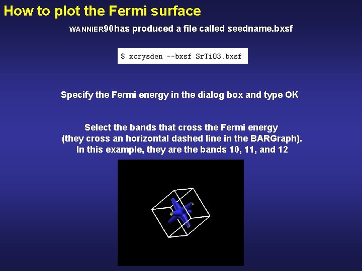
How to plot the Fermi surface WANNIER 90 has produced a file called seedname. bxsf Specify the Fermi energy in the dialog box and type OK Select the bands that cross the Fermi energy (they cross an horizontal dashed line in the BARGraph). In this example, they are the bands 10, 11, and 12

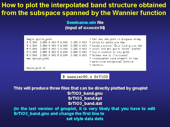
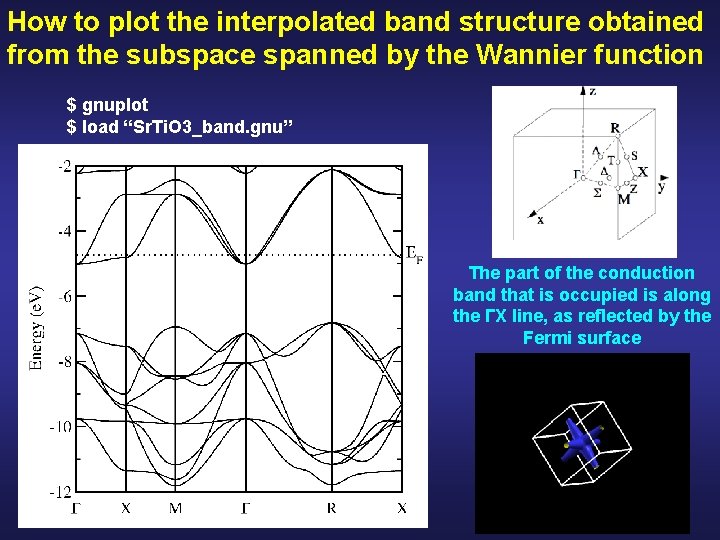
How to plot the interpolated band structure obtained from the subspace spanned by the Wannier function Seedname. win file (input of WANNIER 90) This will produce three files that can be directly plotted by gnuplot Sr. Ti. O 3_band. gnu Sr. Ti. O 3_band. kpt Sr. Ti. O 3_band. dat (in the last version of gnuplot, it is very likely that you have to edit Sr. Ti. O 3_band. gnu and change the first line to set style data dots

How to plot the interpolated band structure obtained from the subspace spanned by the Wannier function $ gnuplot $ load “Sr. Ti. O 3_band. gnu” The part of the conduction band that is occupied is along the ΓX line, as reflected by the Fermi surface

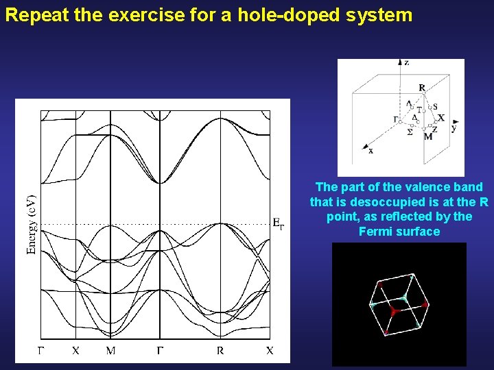
Repeat the exercise for a hole-doped system The part of the valence band that is desoccupied is at the R point, as reflected by the Fermi surface