How to easily simulate a photodetector response Its

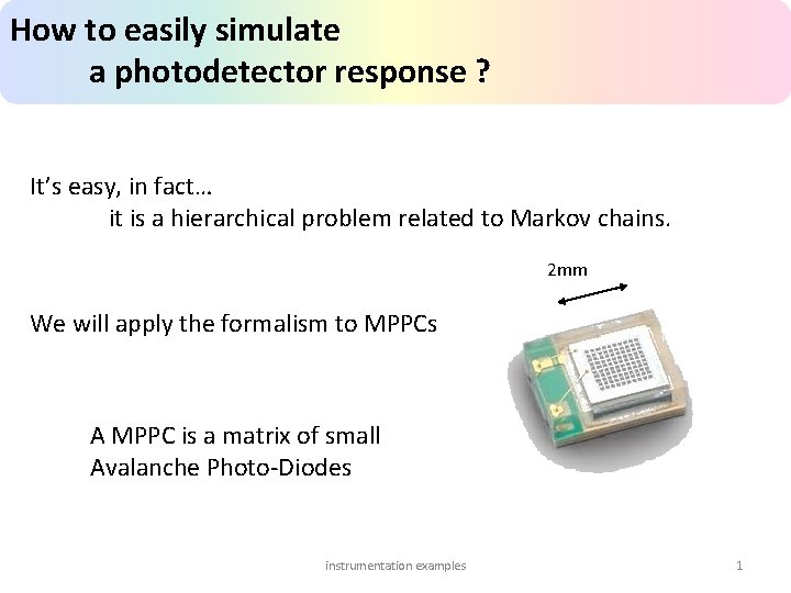
How to easily simulate a photodetector response ? It’s easy, in fact… it is a hierarchical problem related to Markov chains. 2 mm We will apply the formalism to MPPCs A MPPC is a matrix of small Avalanche Photo-Diodes instrumentation examples 1

How to easily simulate a photodetector response ? The MPPC 1. “dark count” is about 1 Mcps 2. When a pixel triggers it has a probability of say 40% to trigger one of its neighbors 3. The single P. E. response is very sharp 4. When a pixel is triggered, it refills at a given rate say 50 ns for instance We will simulate it by using R instrumentation examples 2

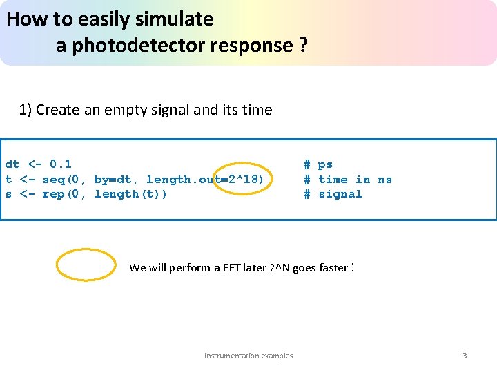
How to easily simulate a photodetector response ? 1) Create an empty signal and its time dt <- 0. 1 t <- seq(0, by=dt, length. out=2^18) s <- rep(0, length(t)) # ps # time in ns # signal We will perform a FFT later 2^N goes faster ! instrumentation examples 3

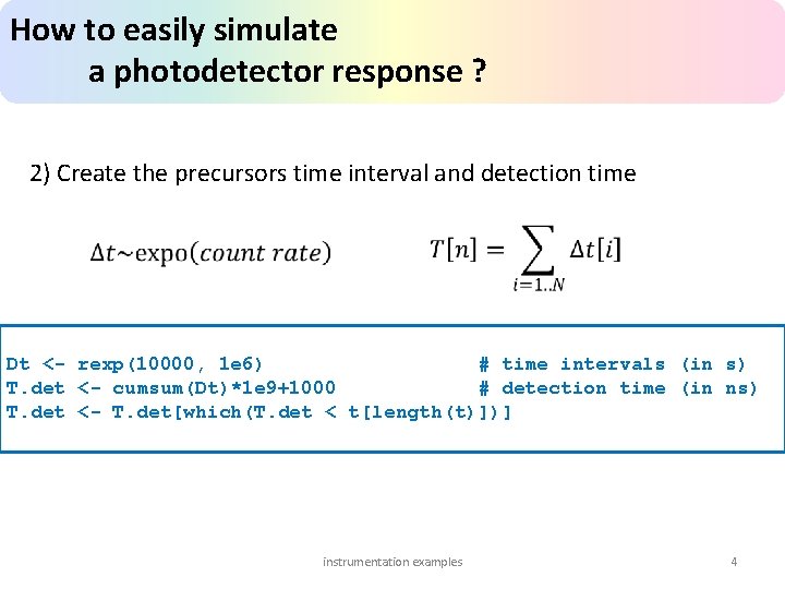
How to easily simulate a photodetector response ? 2) Create the precursors time interval and detection time Dt <- rexp(10000, 1 e 6) # time intervals (in s) T. det <- cumsum(Dt)*1 e 9+1000 # detection time (in ns) T. det <- T. det[which(T. det < t[length(t)])] instrumentation examples 4

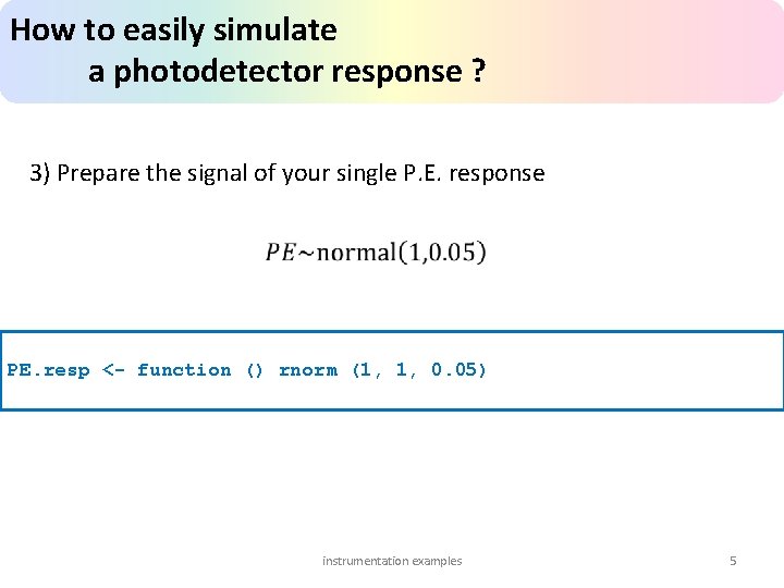
How to easily simulate a photodetector response ? 3) Prepare the signal of your single P. E. response PE. resp <- function () rnorm (1, 1, 0. 05) instrumentation examples 5

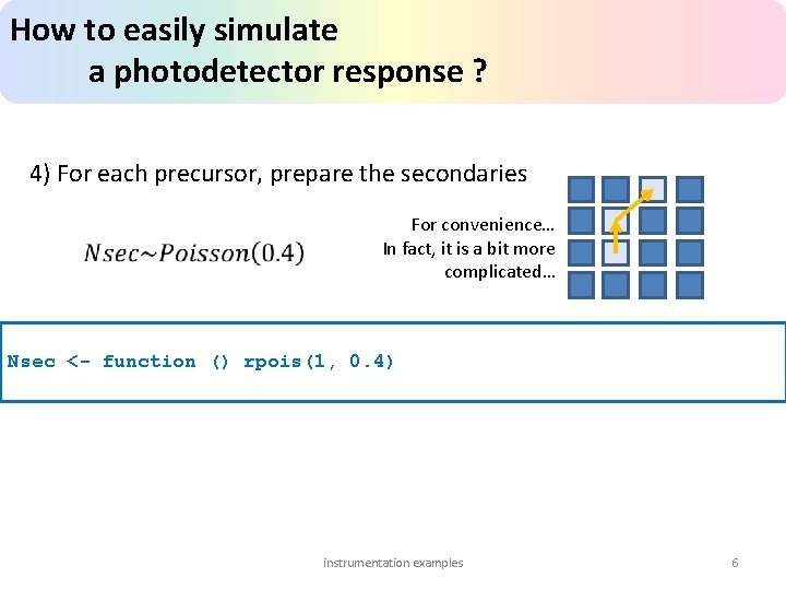
How to easily simulate a photodetector response ? 4) For each precursor, prepare the secondaries For convenience… In fact, it is a bit more complicated… Nsec <- function () rpois(1, 0. 4) instrumentation examples 6

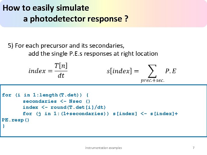
How to easily simulate a photodetector response ? 5) For each precursor and its secondaries, add the single P. E. s responses at right location for (i in 1: length(T. det)) { secondaries <- Nsec () index <- round(T. det[i]/dt) for (j in 1: (1+secondaries)) s[index] <- s[index]+ PE. resp() } instrumentation examples 7

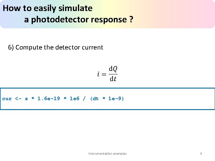
How to easily simulate a photodetector response ? 6) Compute the detector current cur <- s * 1. 6 e-19 * 1 e 6 / (dt * 1 e-9) instrumentation examples 8

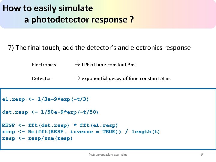
How to easily simulate a photodetector response ? 7) The final touch, add the detector’s and electronics response Electronics LPF of time constant 3 ns Detector exponential decay of time constant 50 ns el. resp <- 1/3 e-9*exp(-t/3) det. resp <- 1/50 e-9*exp(-t/50) RESP <- fft(det. resp) * fft(el. resp) resp <- Re(fft(RESP, inverse = TRUE)) / length(t) resp <- resp/sum(resp) instrumentation examples 9

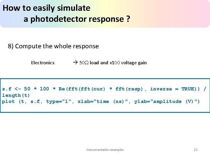
How to easily simulate a photodetector response ? 8) Compute the whole response Electronics 50 W load and x 100 voltage gain s. f <- 50 * 100 * Re(fft(cur) * fft(resp), inverse = TRUE)) / length(t) plot (t, s. f, type="l", xlab="time (ns)", ylab="amplitude (V)") instrumentation examples 10

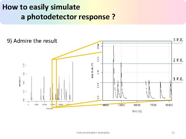
How to easily simulate a photodetector response ? 9) Admire the result 3 P. E. 2 P. E. 1 P. E. instrumentation examples 11

How to easily simulate a photodetector response ? The model is very simple, we could easily add refinements • Better model for secondaries • After pulses • Noise • … Then we would be able to check how this signals enter a given data acquisition system • For time measurements • Amplitude measurements • Dead time… That’s all folks! instrumentation examples 12