How do Climate Models Work What do they

How do Climate Models Work? What do they tell us? Aaron Donohoe Cornish College Lecture 2/26/07

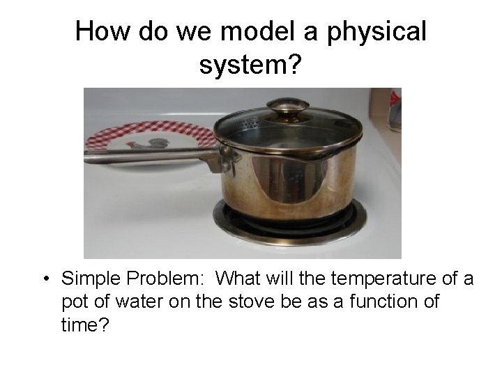
How do we model a physical system? • Simple Problem: What will the temperature of a pot of water on the stove be as a function of time?

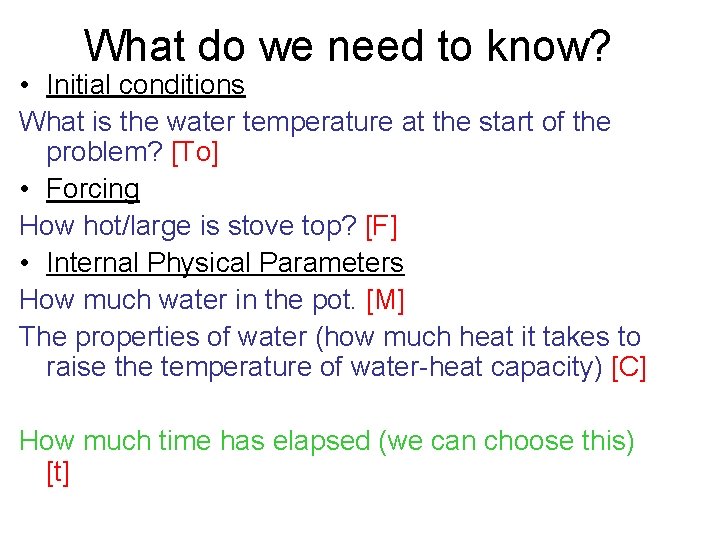
What do we need to know? • Initial conditions What is the water temperature at the start of the problem? [To] • Forcing How hot/large is stove top? [F] • Internal Physical Parameters How much water in the pot. [M] The properties of water (how much heat it takes to raise the temperature of water-heat capacity) [C] How much time has elapsed (we can choose this) [t]

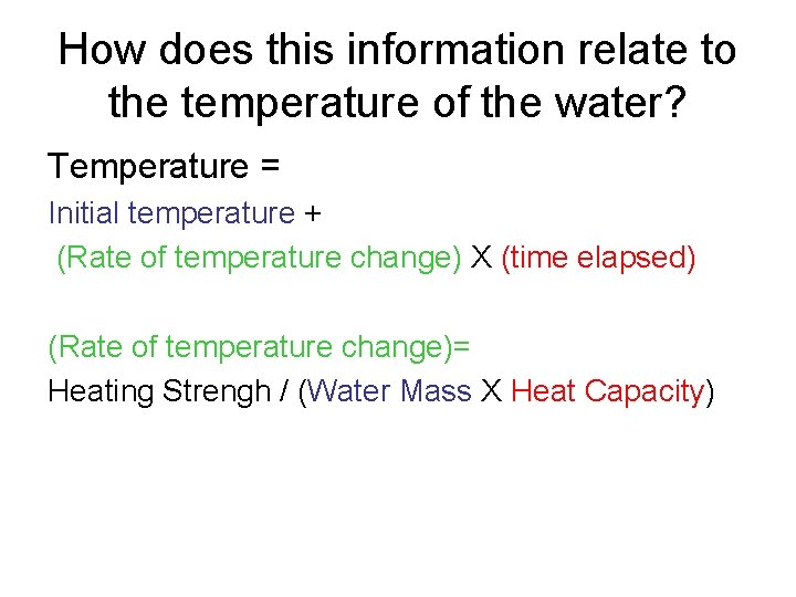
How does this information relate to the temperature of the water? Temperature = Initial temperature + (Rate of temperature change) X (time elapsed) (Rate of temperature change)= Heating Strengh / (Water Mass X Heat Capacity)

Putting it together Initial temperature. [To] How hot/large is stove top? [F] How much water in the pot. [M] Heat capacity of water. [C] How much time has elapsed [t] Temperature [Tf] Tf = To + (F/CM) X t

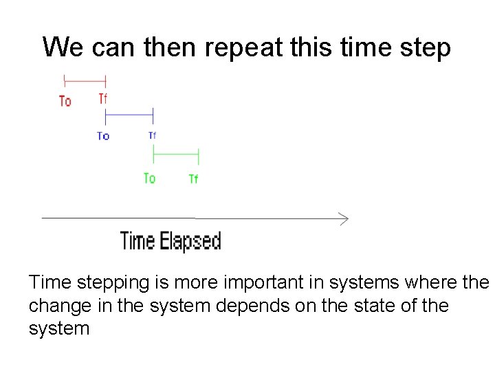
We can then repeat this time step Time stepping is more important in systems where the change in the system depends on the state of the system

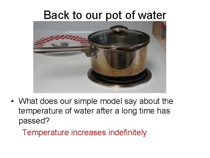
Back to our pot of water • What does our simple model say about the temperature of water after a long time has passed? Temperature increases indefinitely

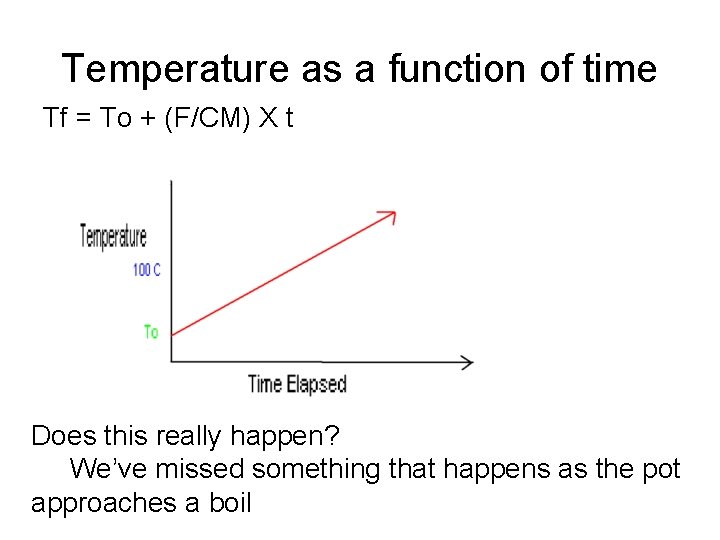
Temperature as a function of time Tf = To + (F/CM) X t Does this really happen? We’ve missed something that happens as the pot approaches a boil

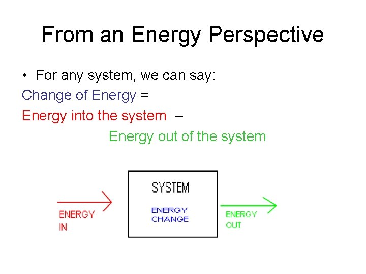
From an Energy Perspective • For any system, we can say: Change of Energy = Energy into the system – Energy out of the system

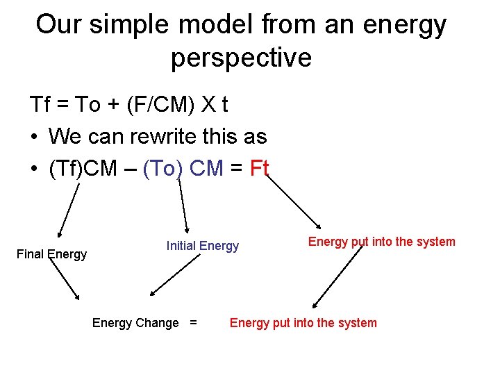
Our simple model from an energy perspective Tf = To + (F/CM) X t • We can rewrite this as • (Tf)CM – (To) CM = Ft Final Energy Initial Energy Change = Energy put into the system

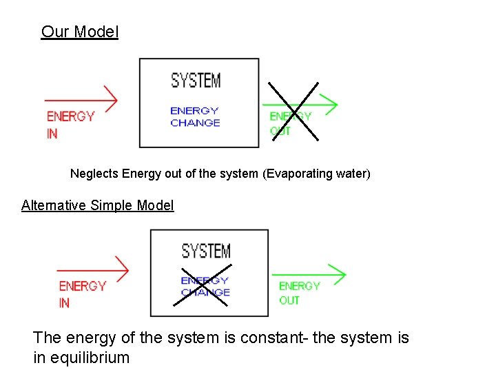
Our Model Neglects Energy out of the system (Evaporating water) Alternative Simple Model The energy of the system is constant- the system is in equilibrium

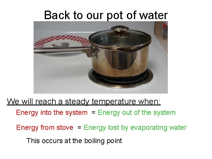
Back to our pot of water We will reach a steady temperature when: Energy into the system = Energy out of the system Energy from stove = Energy lost by evaporating water This occurs at the boiling point

Two different types of models • Transient model The system is evolving • Equilibruim Model The system is in balance- is steady Equilibruim models are useful because they identify the state the system wants to be in

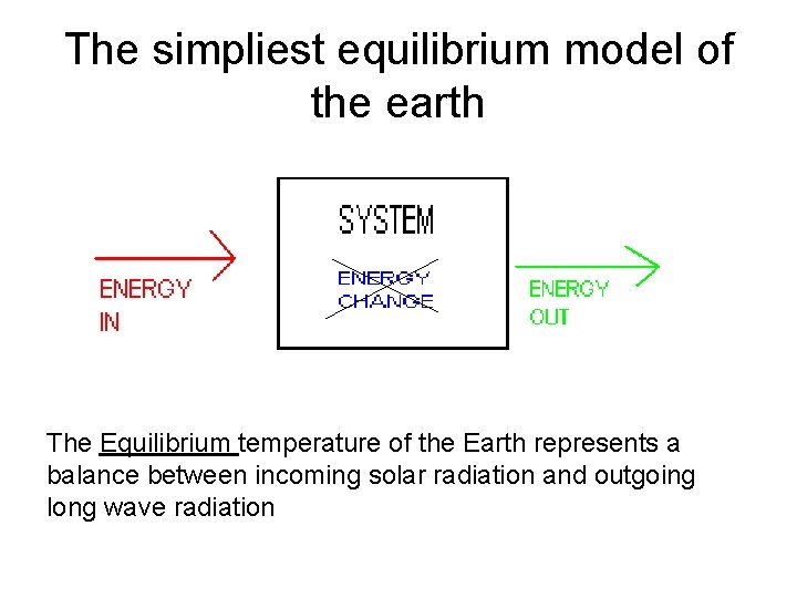
The simpliest equilibrium model of the earth The Equilibrium temperature of the Earth represents a balance between incoming solar radiation and outgoing long wave radiation

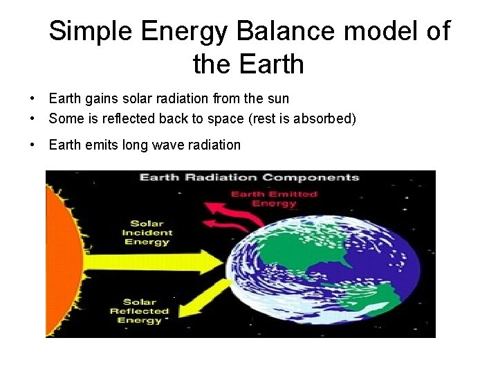
Simple Energy Balance model of the Earth • Earth gains solar radiation from the sun • Some is reflected back to space (rest is absorbed) • Earth emits long wave radiation

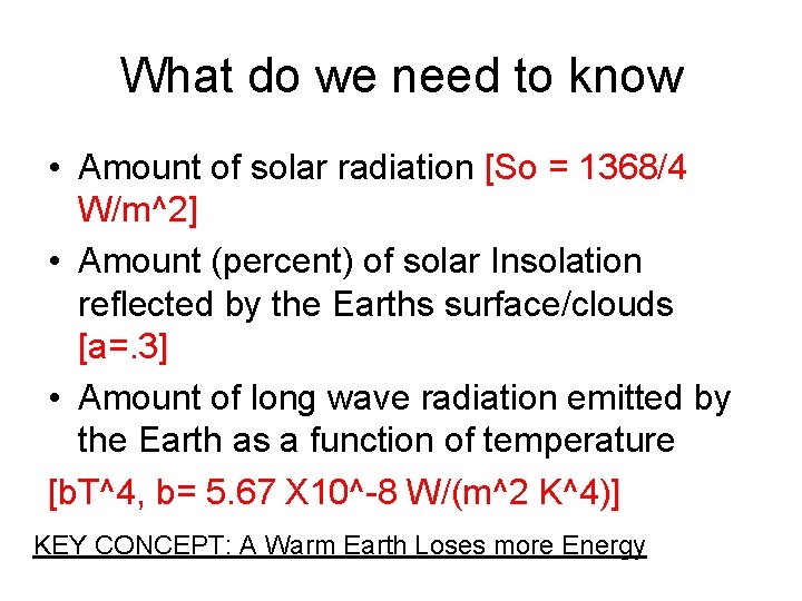
What do we need to know • Amount of solar radiation [So = 1368/4 W/m^2] • Amount (percent) of solar Insolation reflected by the Earths surface/clouds [a=. 3] • Amount of long wave radiation emitted by the Earth as a function of temperature [b. T^4, b= 5. 67 X 10^-8 W/(m^2 K^4)] KEY CONCEPT: A Warm Earth Loses more Energy

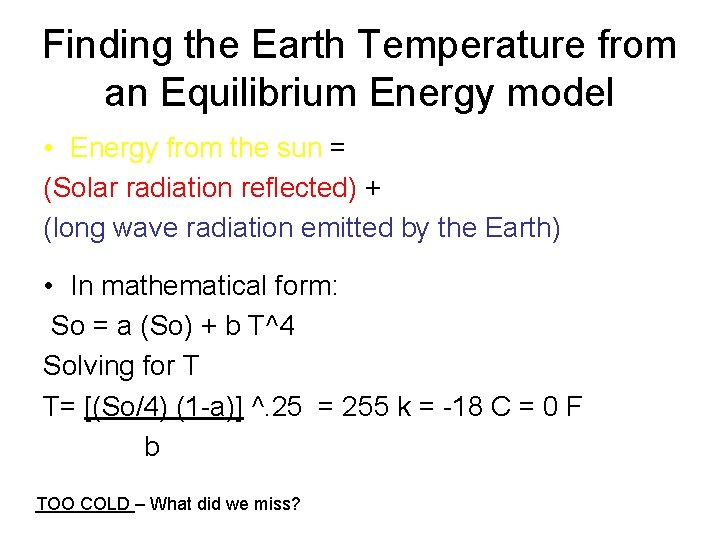
Finding the Earth Temperature from an Equilibrium Energy model • Energy from the sun = (Solar radiation reflected) + (long wave radiation emitted by the Earth) • In mathematical form: So = a (So) + b T^4 Solving for T T= [(So/4) (1 -a)] ^. 25 = 255 k = -18 C = 0 F b TOO COLD – What did we miss?

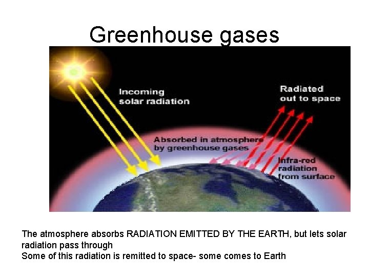
Greenhouse gases The atmosphere absorbs RADIATION EMITTED BY THE EARTH, but lets solar radiation pass through Some of this radiation is remitted to space- some comes to Earth

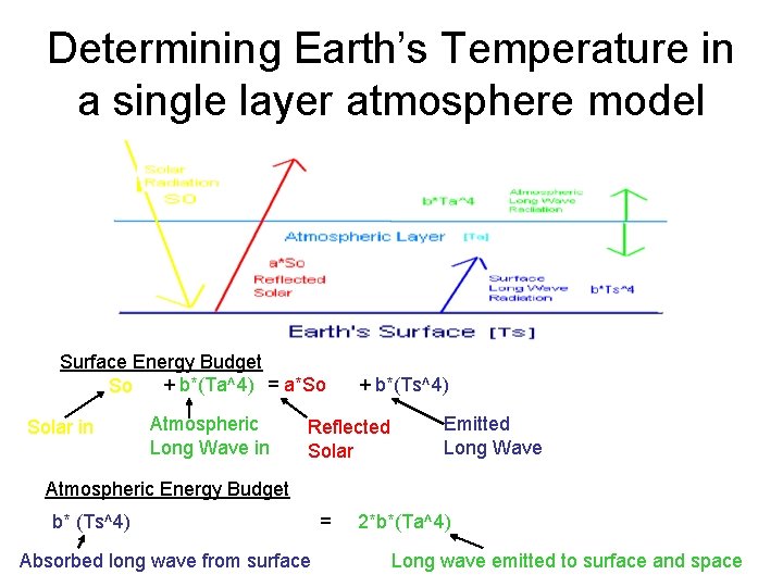
Add a single layer (Greenhouse) to the atmosphere in the model • Solar radiation passes through the atmosphere • Long Wave radiation is absorbed perfectly by the land surface and the atmosphere • The surface and the atmosphere emit long wave radiation according to there temperature

Determining Earth’s Temperature in a single layer atmosphere model Surface Energy Budget + b*(Ta^4) = a*So So Solar in Atmospheric Long Wave in + b*(Ts^4) Reflected Solar Emitted Long Wave Atmospheric Energy Budget b* (Ts^4) Absorbed long wave from surface = 2*b*(Ta^4) Long wave emitted to surface and space

Determining Earth’s Temperature in a single layer atmosphere model • The equations get complicated fairly quickly but • We have reduced the physical system to a mathematical equation • The resulting atmospheric temperature is 50 C • It’s too hot now – what can we do

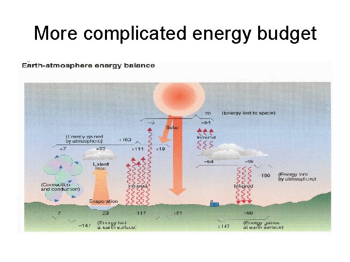
More complicated energy budget

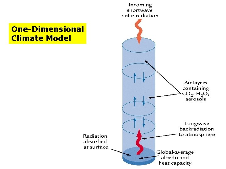
One-Dimensional Climate Model

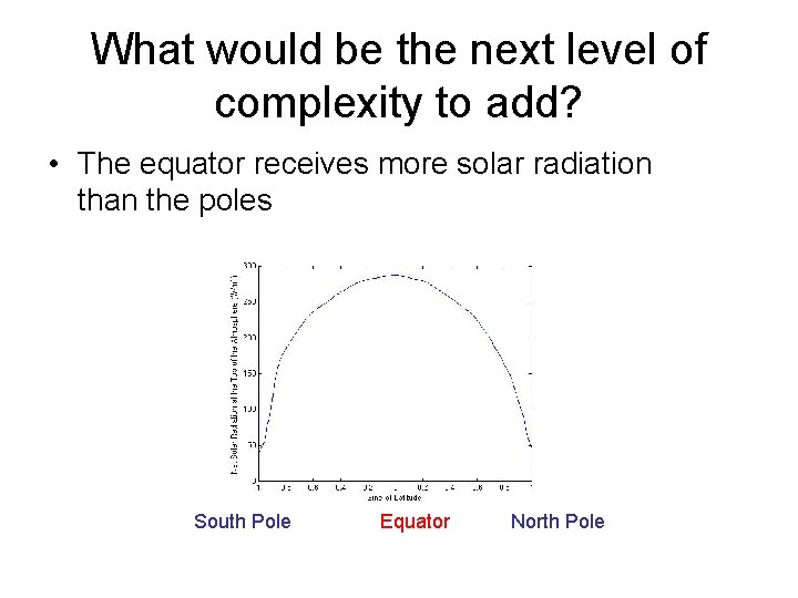
What would be the next level of complexity to add? • The equator receives more solar radiation than the poles South Pole Equator North Pole

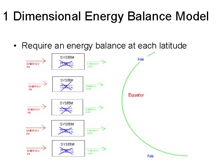
1 Dimensional Energy Balance Model • Require an energy balance at each latitude

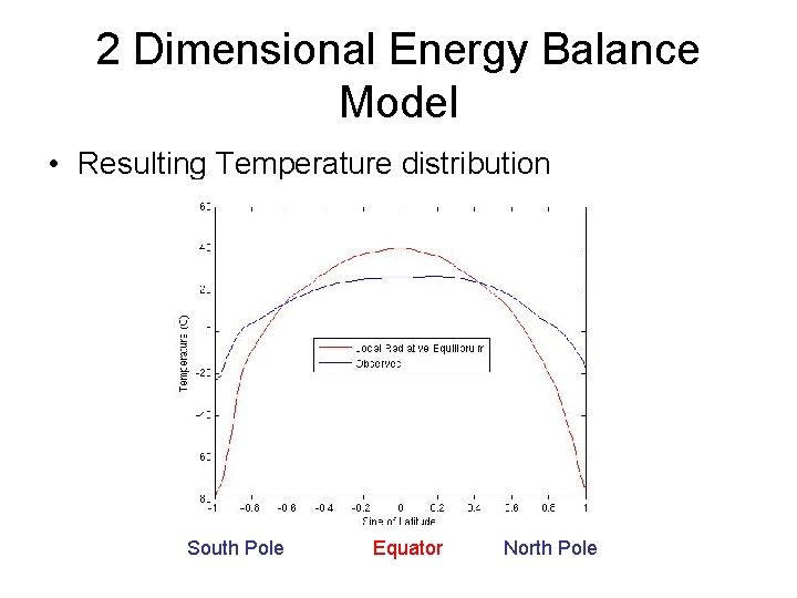
2 Dimensional Energy Balance Model • Resulting Temperature distribution South Pole Equator North Pole

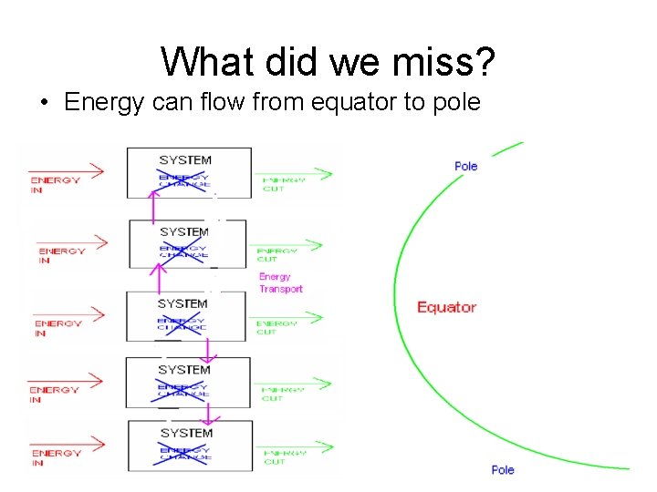
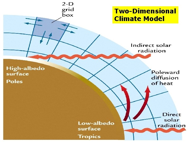
What did we miss? • Energy can flow from equator to pole

Two-Dimensional Climate Model

We must add atmospheric motion • • • % Code up of North and Coakley's seasonal EBM model % Simplified to eliminate the ocean domain % Designed to run without a seasonal cycle and hence % to stop once an equilibrium solution is reached. % The model uses an implicit trapezoidal method % so the timestep can be long. • • %size of domain. jmx=151; • • • % Choose parameters. % scale. Q if (exist('scale. Q')==0); scale. Q=1. ; end • • % OLR constant. if (exist('A')==0); A=203. 3; end • • % OLR coef. if (exist('B')==0); B=2. 09; end • • %heat diffusion coefficient. if (exist('Dmag')==0); Dmag = 0. 44; end • • %heat diffusion coefficient. Toffset=0. ; if (exist('coldstartflag')==1); if (coldstartflag==1), Toffset = -40; end • • %Remove albedo feedback if (exist('albedoflag')==0); albedoflag = 0. ; end • • %heat capacity over land. Cl = 0. 2; % something small to make it equilibriate quickly • • • %time step in fraction of year delt=1. /50; NMAX=1000; • • %set up x array. delx = 2. 0/jmx; x = [-1. 0+delx/2: delx: 1. 0 -delx/2]'; phi = asin(x)*180/pi; • • • %obtain annual array of daily averaged- insolation. %[insol] = sun(x); %Legendre polynomial realizatin of mean annual insol. if (exist('S')==1); S=S; %Simulate Hadley Cell with Lindzen and Farrell plan if (exist('hadleyflag')==0); hadleyflag = 0. ; end

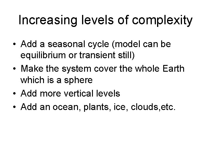
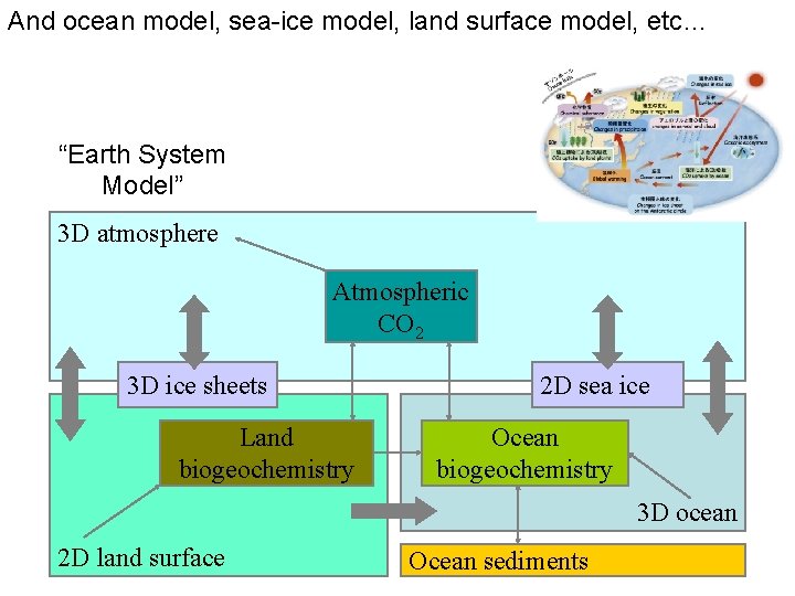
Increasing levels of complexity • Add a seasonal cycle (model can be equilibrium or transient still) • Make the system cover the whole Earth which is a sphere • Add more vertical levels • Add an ocean, plants, ice, clouds, etc.

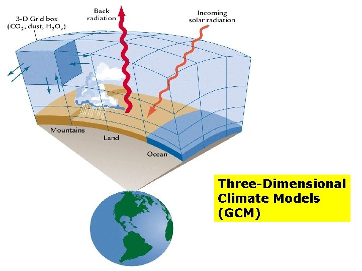
Three-Dimensional Climate Models (GCM)

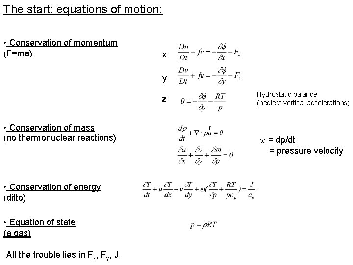
The start: equations of motion: • Conservation of momentum (F=ma) x y z • Conservation of mass (no thermonuclear reactions) • Conservation of energy (ditto) • Equation of state (a gas) All the trouble lies in Fx, Fy, J Hydrostatic balance (neglect vertical accelerations) = dp/dt = pressure velocity

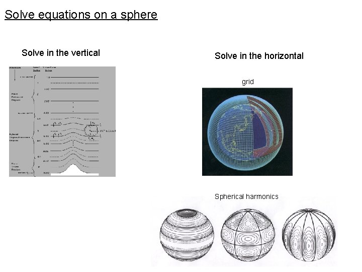
Solve equations on a sphere Solve in the vertical Solve in the horizontal grid Spherical harmonics

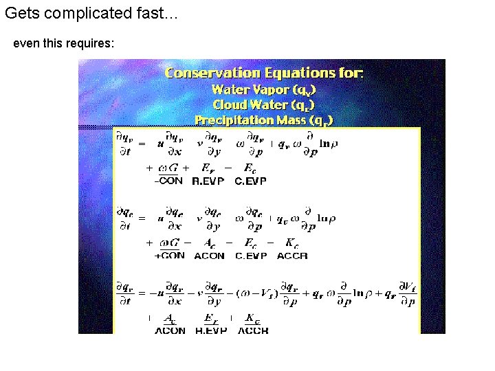
Gets complicated fast… Begin to think about clouds

Gets complicated fast… even this requires:

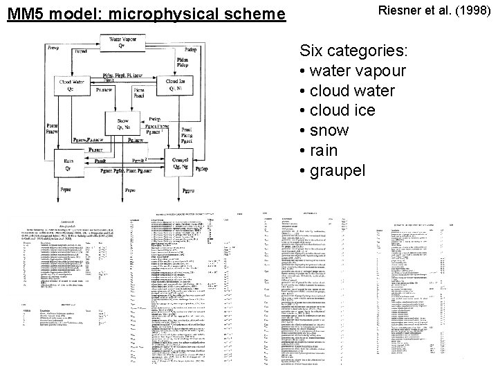
MM 5 model: microphysical scheme Riesner et al. (1998) Six categories: • water vapour • cloud water • cloud ice • snow • rain • graupel

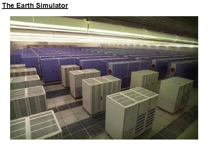
The Earth Simulator

Not just the atmosphere…

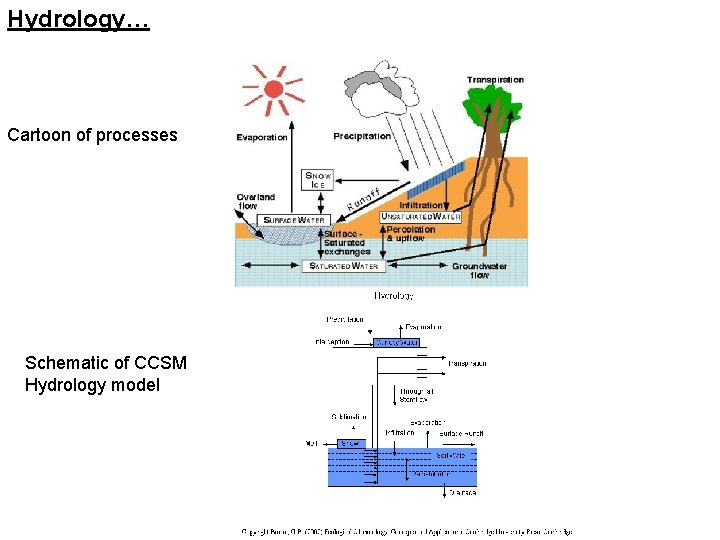
Hydrology… Cartoon of processes Schematic of CCSM Hydrology model

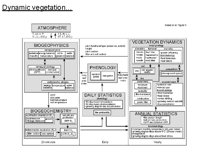
Dynamic vegetation…

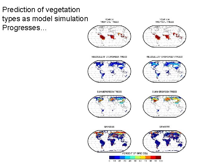
Prediction of vegetation types as model simulation Progresses…

And ocean model, sea-ice model, land surface model, etc… “Earth System Model” 3 D atmosphere Atmospheric CO 2 3 D ice sheets Land biogeochemistry 2 D sea ice Ocean biogeochemistry 3 D ocean 2 D land surface Ocean sediments

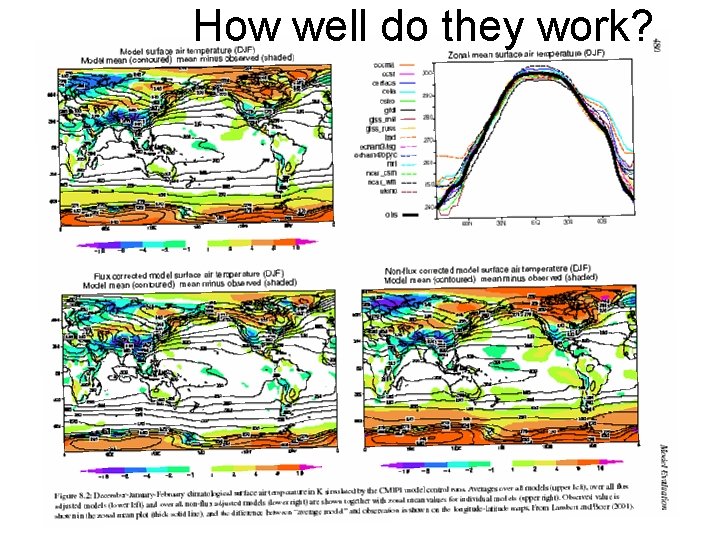
How well do they work?

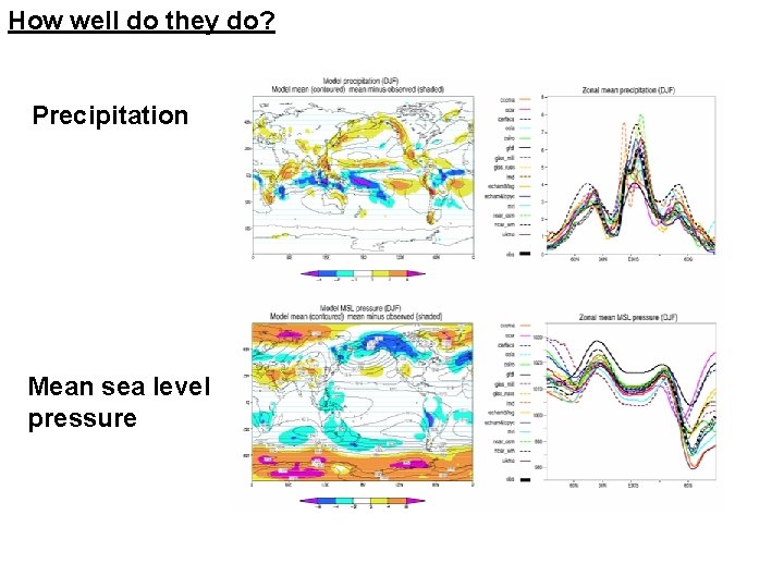
How well do they do? Precipitation Mean sea level pressure

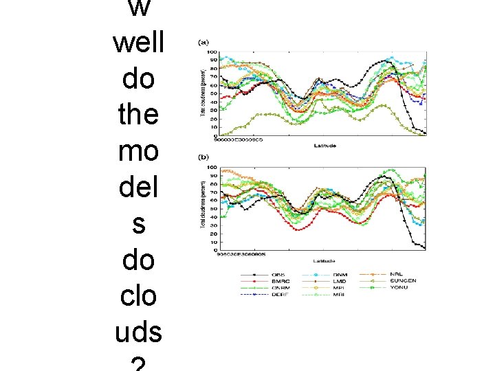
w well do the mo del s do clo uds

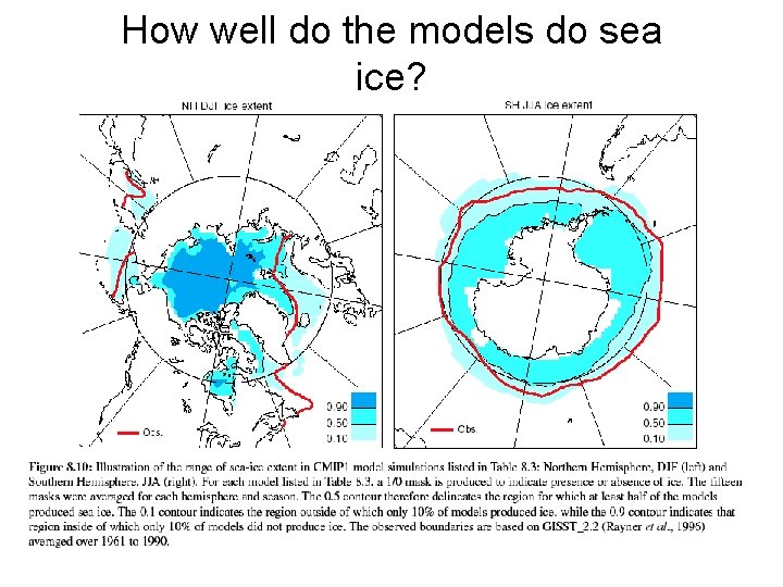
How well do the models do sea ice?

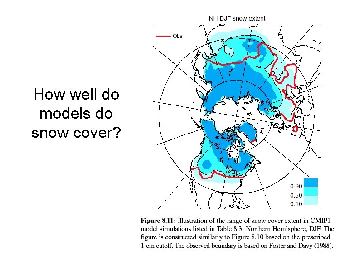
How well do models do snow cover?

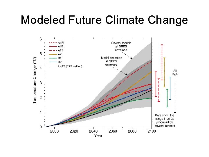
Modeled Future Climate Change

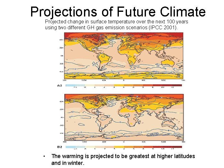
Projections of Future Climate Projected change in surface temperature over the next 100 years using two different GH gas emission scenarios (IPCC 2001). • The warming is projected to be greatest at higher latitudes and in winter.

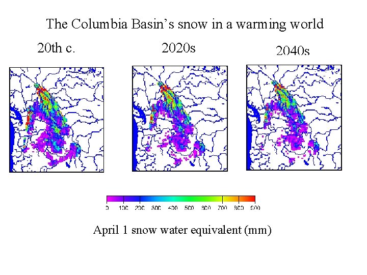
The Columbia Basin’s snow in a warming world 20 th c. 2020 s April 1 snow water equivalent (mm) 2040 s