How Computers Work Lecture 12 Introduction to Pipelining

How Computers Work Lecture 12 Introduction to Pipelining How Computers Work Lecture 12 Page 1

A Common Chore of College Life How Computers Work Lecture 12 Page 2

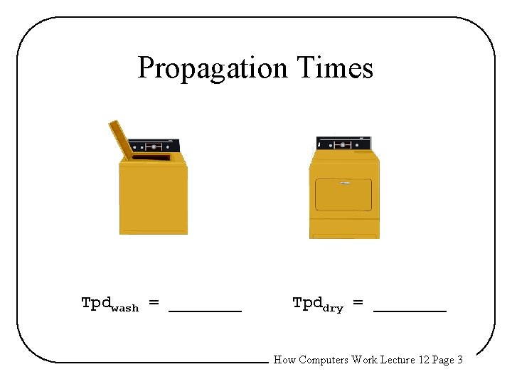
Propagation Times Tpdwash = _______ Tpddry = _______ How Computers Work Lecture 12 Page 3

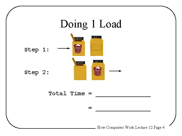
Doing 1 Load Step 1: Step 2: Total Time = _______________ How Computers Work Lecture 12 Page 4

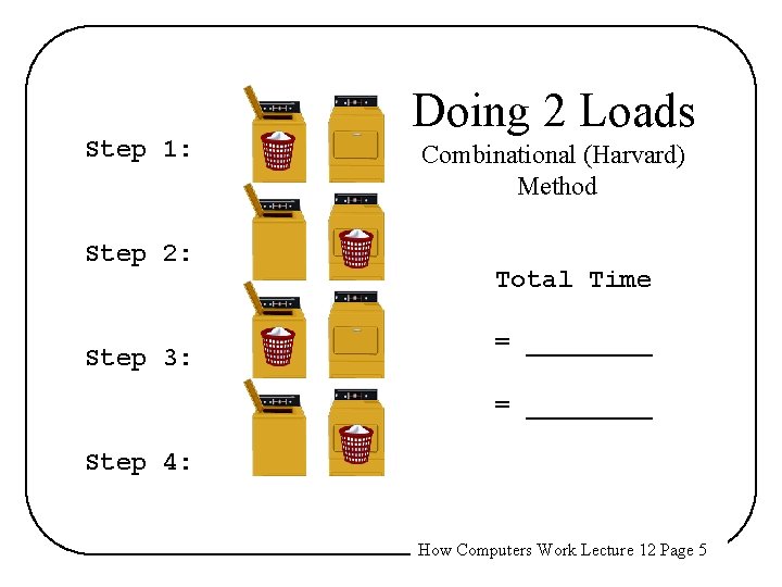
Step 1: Step 2: Step 3: Doing 2 Loads Combinational (Harvard) Method Total Time = ________ Step 4: How Computers Work Lecture 12 Page 5

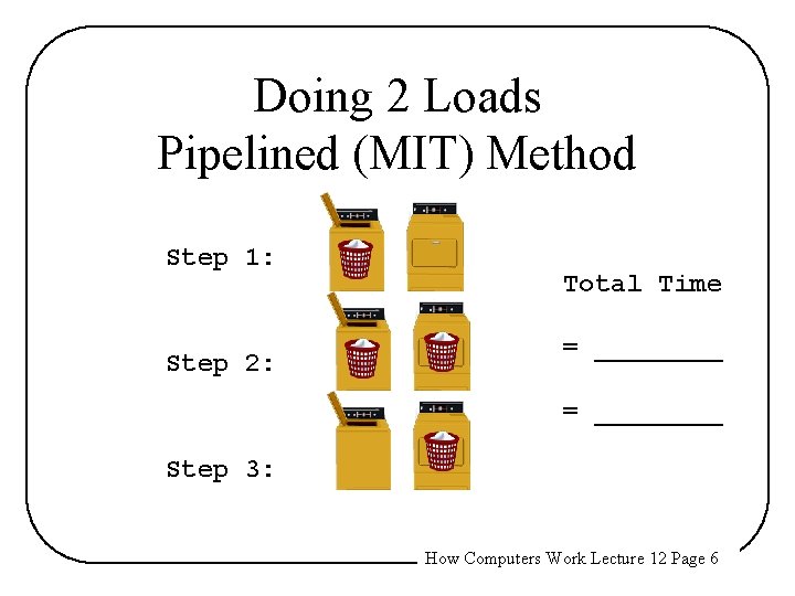
Doing 2 Loads Pipelined (MIT) Method Step 1: Step 2: Total Time = ________ Step 3: How Computers Work Lecture 12 Page 6

Doing N Loads • Harvard Method: _________ • MIT Method: __________ How Computers Work Lecture 12 Page 7

A Few Definitions Latency: Time for 1 object to pass through entire system. (= ____ for Harvard laundry) (= ____ for MIT laundry) Throughput: Rate of objects going through. (= ____ for Harvard laundry) (= ____ for MIT laundry) How Computers Work Lecture 12 Page 8

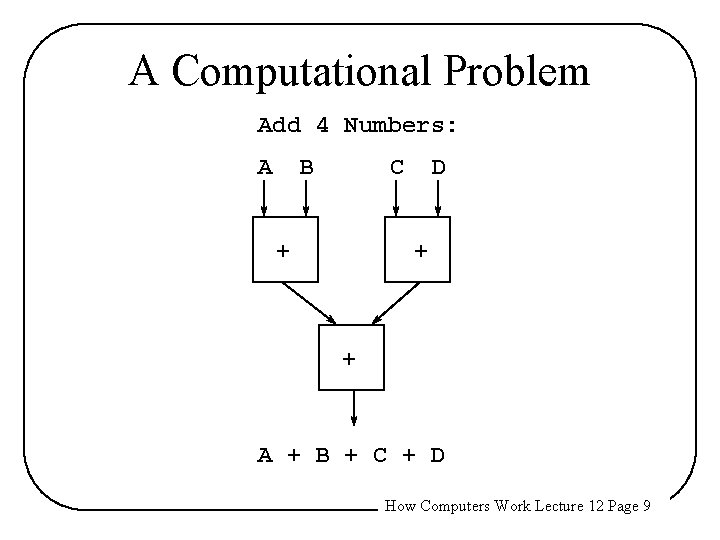
A Computational Problem Add 4 Numbers: A B C + D + + A + B + C + D How Computers Work Lecture 12 Page 9

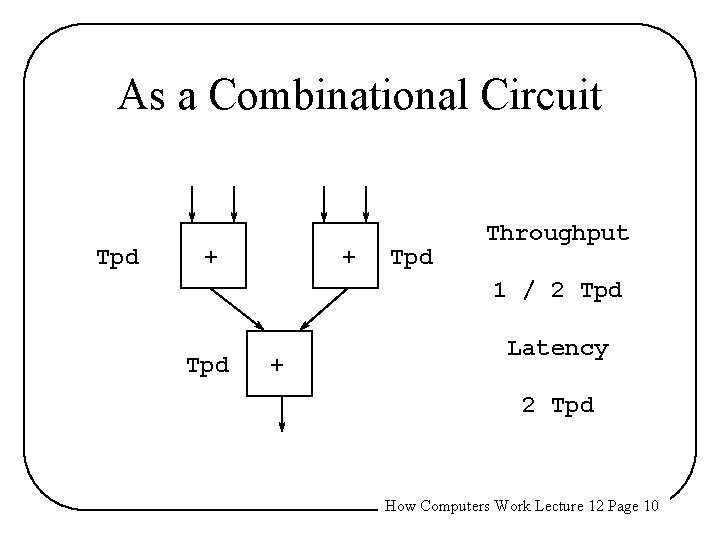
As a Combinational Circuit Tpd + + Tpd Throughput 1 / 2 Tpd + Latency 2 Tpd How Computers Work Lecture 12 Page 10

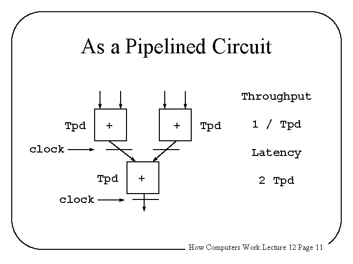
As a Pipelined Circuit Throughput Tpd + + clock Tpd 1 / Tpd Latency Tpd + 2 Tpd clock How Computers Work Lecture 12 Page 11

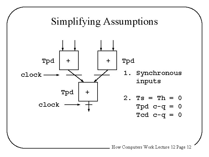
Simplifying Assumptions Tpd + + 1. Synchronous inputs clock Tpd + 2. Ts = Th = 0 Tpd c-q = 0 Tcd c-q = 0 How Computers Work Lecture 12 Page 12

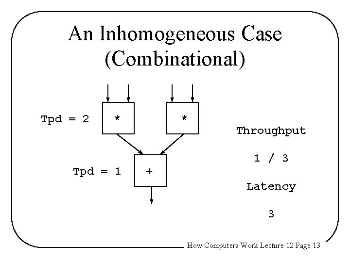
An Inhomogeneous Case (Combinational) Tpd = 2 * Tpd = 1 * + Throughput 1 / 3 Latency 3 How Computers Work Lecture 12 Page 13

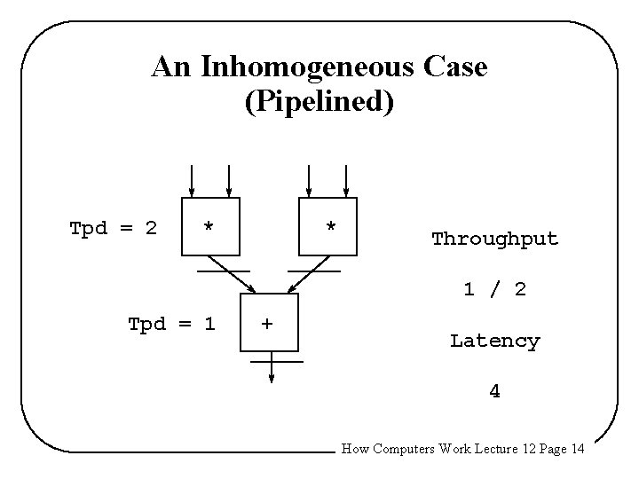
An Inhomogeneous Case (Pipelined) Tpd = 2 * * Throughput 1 / 2 Tpd = 1 + Latency 4 How Computers Work Lecture 12 Page 14

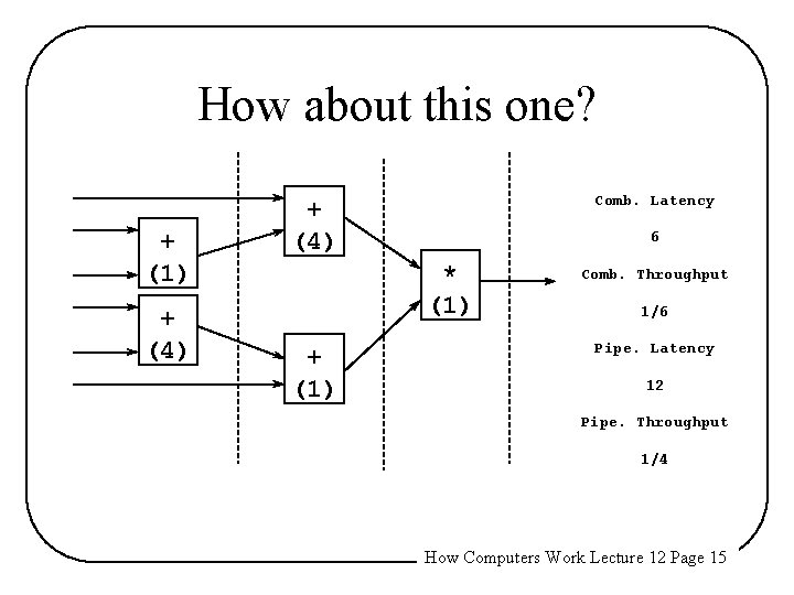
How about this one? + (1) + (4) Comb. Latency + (4) 6 * (1) + (1) Comb. Throughput 1/6 Pipe. Latency 12 Pipe. Throughput 1/4 How Computers Work Lecture 12 Page 15

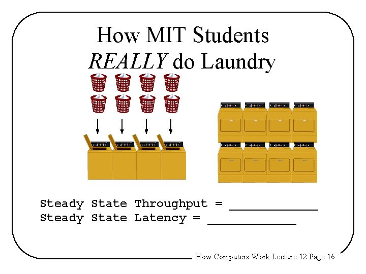
How MIT Students REALLY do Laundry Steady State Throughput = ______ Steady State Latency = ______ How Computers Work Lecture 12 Page 16

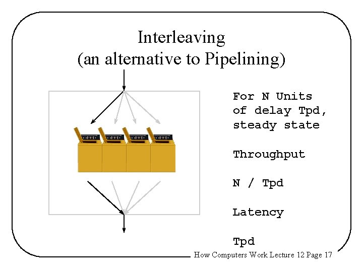
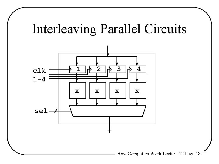
Interleaving (an alternative to Pipelining) For N Units of delay Tpd, steady state Throughput N / Tpd Latency Tpd How Computers Work Lecture 12 Page 17

Interleaving Parallel Circuits clk 1 -4 1 2 3 4 x x sel How Computers Work Lecture 12 Page 18

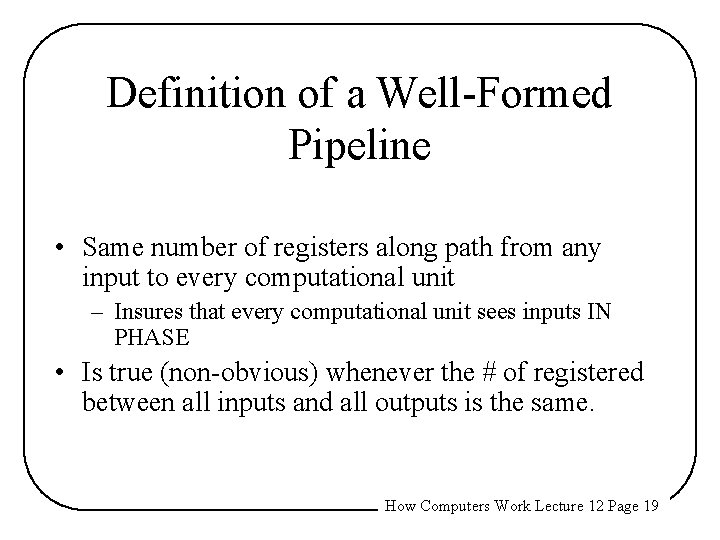
Definition of a Well-Formed Pipeline • Same number of registers along path from any input to every computational unit – Insures that every computational unit sees inputs IN PHASE • Is true (non-obvious) whenever the # of registered between all inputs and all outputs is the same. How Computers Work Lecture 12 Page 19

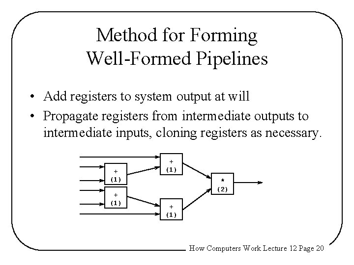
Method for Forming Well-Formed Pipelines • Add registers to system output at will • Propagate registers from intermediate outputs to intermediate inputs, cloning registers as necessary. + (1) * (2) + (1) How Computers Work Lecture 12 Page 20

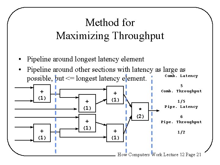
Method for Maximizing Throughput • Pipeline around longest latency element • Pipeline around other sections with latency as large as Comb. Latency possible, but <= longest latency element. + (1) 5 Comb. Throughput + (1) * (2) + (1) 1/5 Pipe. Latency 6 Pipe. Throughput 1/2 How Computers Work Lecture 12 Page 21

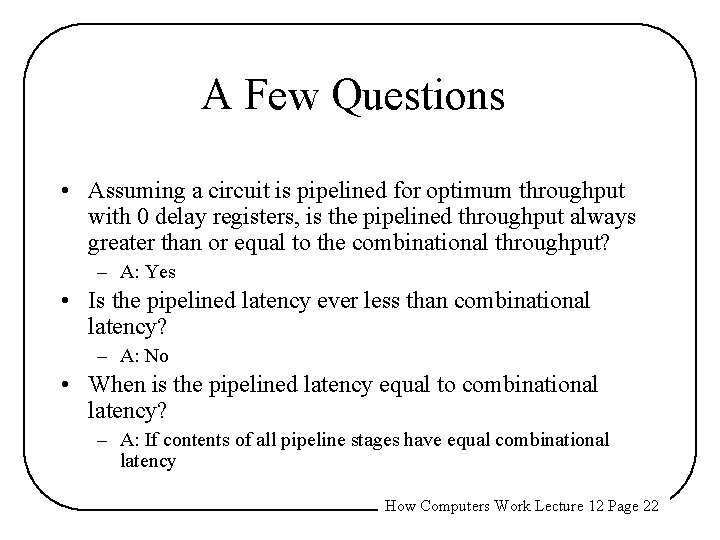
A Few Questions • Assuming a circuit is pipelined for optimum throughput with 0 delay registers, is the pipelined throughput always greater than or equal to the combinational throughput? – A: Yes • Is the pipelined latency ever less than combinational latency? – A: No • When is the pipelined latency equal to combinational latency? – A: If contents of all pipeline stages have equal combinational latency How Computers Work Lecture 12 Page 22

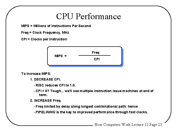
CPU Performance MIPS = Millions of Instructions Per Second Freq = Clock Frequency, MHz CPI = Clocks per Instruction MIPS = Freq CPI To Increase MIPS: 1. DECREASE CPI. - RISC reduces CPI to 1. 0. - CPI < 0? Tough. . . we’ll see multiple instruction issue machines at end of term. 2. INCREASE Freq. - Freq limited by delay alongest combinational path; hence - PIPELINING is the key to improved performance through fast clocks. How Computers Work Lecture 12 Page 23

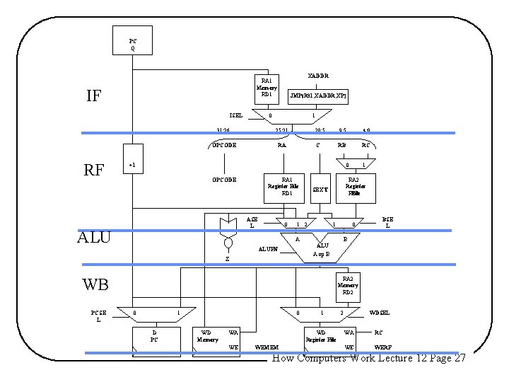
Review: A Top-Down View of the Beta Architecture With st(ra, C, rc) : Mem[C+<rc>] <- <ra> PC Q XADDR RA 1 Memory RD 1 ISEL JMP(R 31, XADDR, XP) 0 1 31: 26 25: 21 OPCODE RA 20: 5 9: 5 4: 0 C RB RC +1 0 RA 1 Register File RD 1 OPCODE ASEL 0 1 RA 2 Register File RD 2 SEXT 2 1 1 0 A BSEL B ALU A op B ALUFN Z RA 2 Memory RD 2 PCSEL 0 1 D PC 0 WD Memory WA WE WEMEM 1 WD Register File 2 WDSEL WA RC WE WERF How Computers Work Lecture 12 Page 24

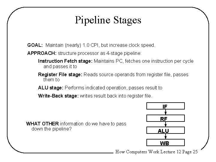
Pipeline Stages GOAL: Maintain (nearly) 1. 0 CPI, but increase clock speed. APPROACH: structure processor as 4 -stage pipeline: Instruction Fetch stage: Maintains PC, fetches one instruction per cycle and passes it to Register File stage: Reads source operands from register file, passes them to ALU stage: Performs indicated operation, passes result to Write-Back stage: writes result back into register file. IF WHAT OTHER information do we have to pass down the pipeline? RF ALU WB How Computers Work Lecture 12 Page 25

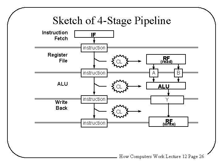
Sketch of 4 -Stage Pipeline Instruction Fetch IF instruction Register File instruction ALU Write Back RF CL (read) A CL instruction B ALU Y CL instruction RF (write) How Computers Work Lecture 12 Page 26

PC Q IF ISEL RF XADDR RA 1 Memory RD 1 JMP(R 31, XADDR, XP) 0 1 31: 26 25: 21 OPCODE RA 20: 5 9: 5 4: 0 C RB RC +1 0 OPCODE RA 1 Register File RD 1 ASE L ALU 0 RA 2 Register File RD 2 SEXT 1 2 1 0 A BSE L B ALU A op B ALUFN Z WB PCSE L 1 RA 2 Memory RD 2 0 1 D PC 0 WD Memory WD Register File WA WE 1 WEMEM 2 WDSEL WA RC WE WERF How Computers Work Lecture 12 Page 27

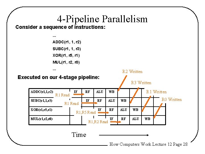
4 -Pipeline Parallelism Consider a sequence of instructions: . . . ADDC(r 1, 1, r 2) SUBC(r 1, 1, r 3) XOR(r 1, r 5, r 1) MUL(r 1, r 2, r 0). . . R 2 Written Executed on our 4 -stage pipeline: R 3 Written ADDC(r 1, 1, r 2) SUBC(r 1, 1, r 3) XOR(r 1, r 5, r 1) R 1 Read IF R 1 Read R 1 Written RF ALU WB IF RF ALU R 1, R 5 Read MUL(r 1, r 2, r 0) R 1, R 2 Read R 0 Written WB Time How Computers Work Lecture 12 Page 28

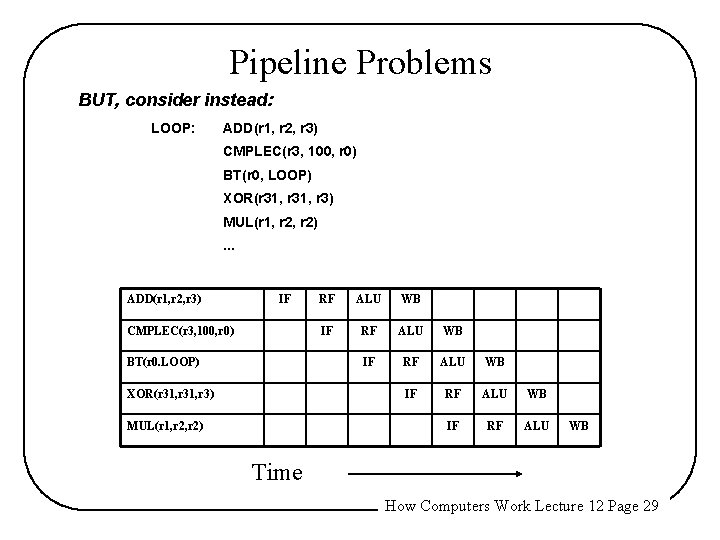
Pipeline Problems BUT, consider instead: LOOP: ADD(r 1, r 2, r 3) CMPLEC(r 3, 100, r 0) BT(r 0, LOOP) XOR(r 31, r 3) MUL(r 1, r 2). . . ADD(r 1, r 2, r 3) IF CMPLEC(r 3, 100, r 0) BT(r 0. LOOP) XOR(r 31, r 3) MUL(r 1, r 2) RF ALU WB IF RF ALU WB Time How Computers Work Lecture 12 Page 29

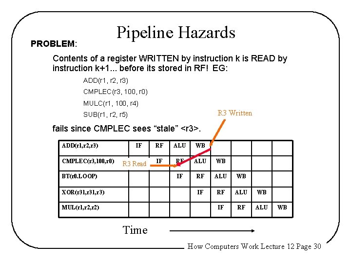
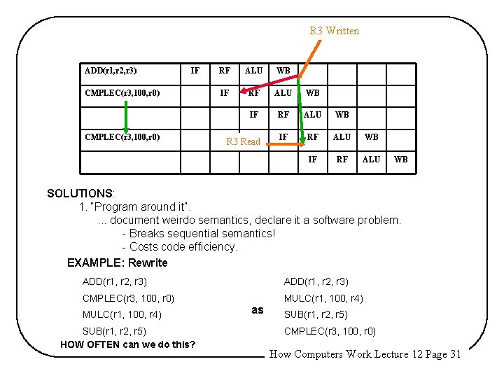
Pipeline Hazards PROBLEM: Contents of a register WRITTEN by instruction k is READ by instruction k+1. . . before its stored in RF! EG: ADD(r 1, r 2, r 3) CMPLEC(r 3, 100, r 0) MULC(r 1, 100, r 4) R 3 Written SUB(r 1, r 2, r 5) fails since CMPLEC sees “stale” <r 3>. ADD(r 1, r 2, r 3) CMPLEC(r 3, 100, r 0) IF R 3 Read BT(r 0. LOOP) XOR(r 31, r 3) MUL(r 1, r 2) RF ALU WB IF RF ALU WB Time How Computers Work Lecture 12 Page 30

R 3 Written ADD(r 1, r 2, r 3) IF CMPLEC(r 3, 100, r 0) RF ALU WB IF RF ALU WB R 3 Read IF RF ALU WB SOLUTIONS: 1. “Program around it”. . document weirdo semantics, declare it a software problem. - Breaks sequential semantics! - Costs code efficiency. EXAMPLE: Rewrite ADD(r 1, r 2, r 3) CMPLEC(r 3, 100, r 0) MULC(r 1, 100, r 4) SUB(r 1, r 2, r 5) HOW OFTEN can we do this? as SUB(r 1, r 2, r 5) CMPLEC(r 3, 100, r 0) How Computers Work Lecture 12 Page 31

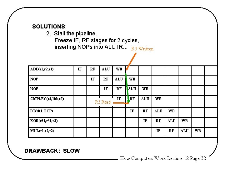
SOLUTIONS: 2. Stall the pipeline. Freeze IF, RF stages for 2 cycles, inserting NOPs into ALU IR. . . R 3 Written ADD(r 1, r 2, r 3) IF NOP CMPLEC(r 3, 100, r 0) BT(r 0. LOOP) XOR(r 31, r 3) MUL(r 1, r 2) RF ALU WB IF RF ALU WB IF RF ALU R 3 Read WB DRAWBACK: SLOW How Computers Work Lecture 12 Page 32

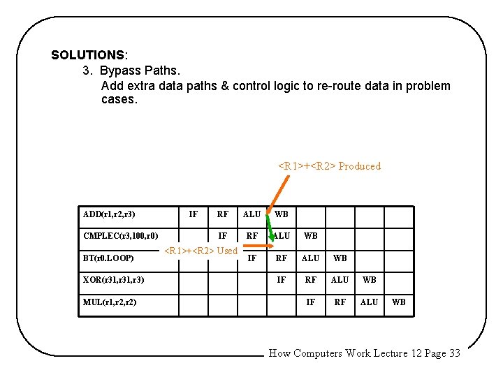
SOLUTIONS: 3. Bypass Paths. Add extra data paths & control logic to re-route data in problem cases. <R 1>+<R 2> Produced ADD(r 1, r 2, r 3) CMPLEC(r 3, 100, r 0) BT(r 0. LOOP) XOR(r 31, r 3) MUL(r 1, r 2) IF RF ALU WB IF RF ALU <R 1>+<R 2> Used WB How Computers Work Lecture 12 Page 33

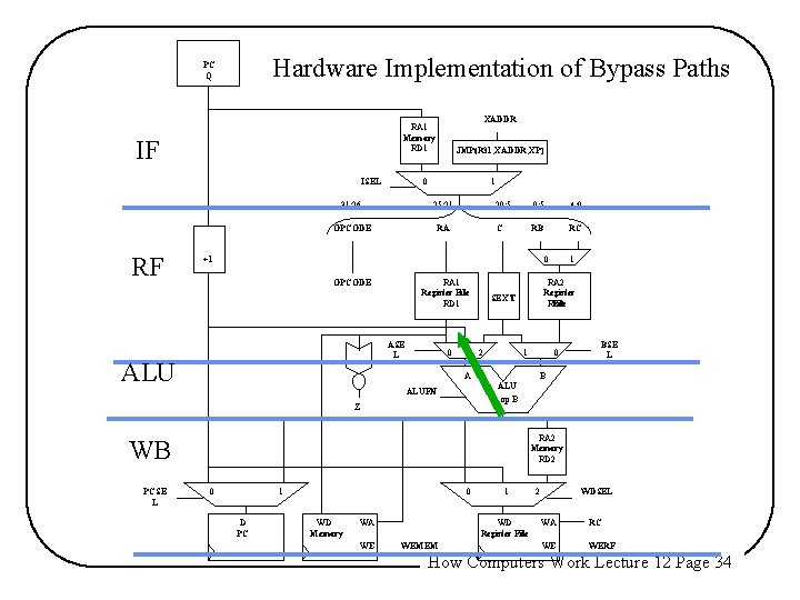
Hardware Implementation of Bypass Paths PC Q IF ISEL RF XADDR RA 1 Memory RD 1 JMP(R 31, XADDR, XP) 0 1 31: 26 25: 21 OPCODE RA 20: 5 9: 5 4: 0 C RB RC +1 0 OPCODE RA 1 Register File RD 1 ASE L ALU 0 RA 2 Register File RD 2 SEXT 1 2 1 0 A BSE L B ALU A op B ALUFN Z RA 2 Memory RD 2 WB PCSE L 1 0 1 D PC 0 WD Memory WD Register File WA WE 1 WEMEM 2 WDSEL WA RC WE WERF How Computers Work Lecture 12 Page 34

Next Time: • Detailed Design of – Bypass Paths + Control Logic • What to do when Bypass Paths Don’t Work – Branch Delays / Tradeoffs – Load/Store Delays / Tradeoffs – Multi-Stage Memory Pipeline How Computers Work Lecture 12 Page 35